CHOOSING A MODEL OF COMPUTATION 4 2 CHOOSING

CHOOSING A MODEL OF COMPUTATION

4. 2 CHOOSING A MODEL OF COMPUTATION TURING machine REGISTER machine 1. 2. They have equivalent power in terms of absolute computability (when resource bounds are not considered. ) They are polynomially related in terms of their effect on running time and space. A choice between these models has no importance from the point of view of tractability/intractability.

4. 2. 1 ISSUES OF COMPUTABILITY Major questions: 1. Computability: “What kind of problem can be solved on a given model of computation”? 2. Complexity: “Can the same problem be solved in polynomial time on all reasonable models of computation”? 1) Most of the problems are UNSOLVABLE D) HALTING PROBLEM: “Does there exist an algorithm which, given two bit strings, the first representing a program and the second representing data determines whether or not the program that runs on the data will stop”?

4. 2. 1 ISSUES OF COMPUTABILITY CONT’D D) HALTING PROBLEM: Ξ “Does the program return the correct answer”? Proof pag. 98 - is by diagonalization ! S) The existence of unsolvable problems led in 1930 s to the study of computability, starting with the design of the universal models of computation. D) A universal model of computation – is a model capable of carrying out any algorithmic process. Models developed from math, logic. , and psychology. - All models proved to be equivalent from computability point of view (what one can compute, all others can too). => Models are universal.

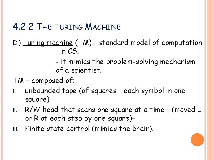
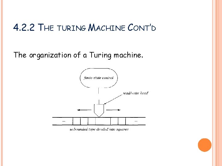
4. 2. 2 THE TURING MACHINE D) Turing machine (TM) – standard model of computation in CS. - it mimics the problem-solving mechanism of a scientist. TM – composed of: i. unbounded tape (of squares – each symbol in one square) ii. R/W head that scans one square at a time – (moved L or R at each step by one square)iii. Finite state control (mimics the brain).

4. 2. 2 THE TURING MACHINE CONT’D The organization of a Turing machine.

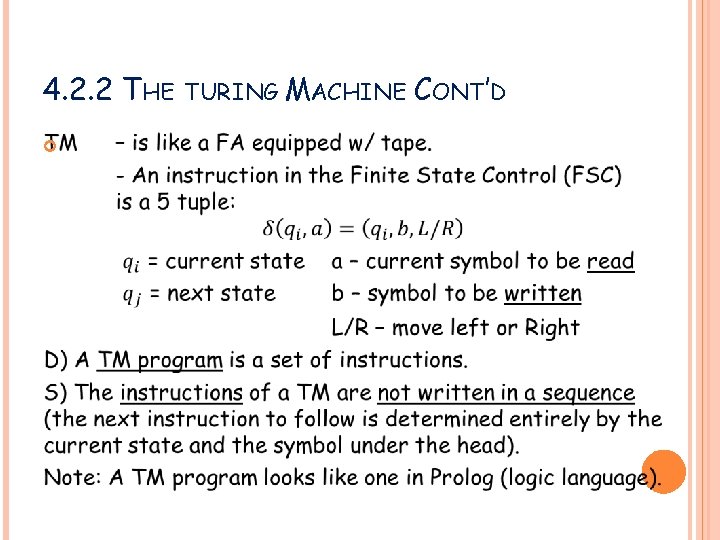
4. 2. 2 THE TURING MACHINE CONT’D

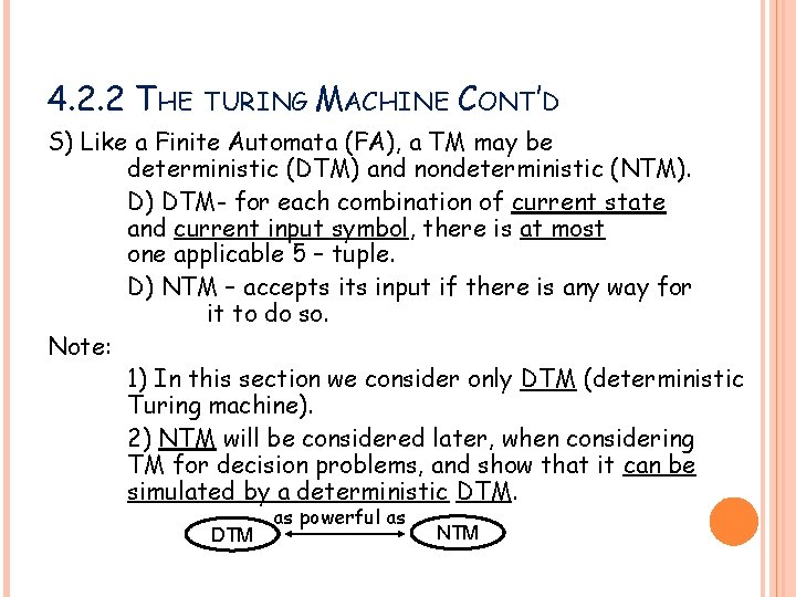
4. 2. 2 THE TURING MACHINE CONT’D S) Like a Finite Automata (FA), a TM may be deterministic (DTM) and nondeterministic (NTM). D) DTM- for each combination of current state and current input symbol, there is at most one applicable 5 – tuple. D) NTM – accepts input if there is any way for it to do so. Note: 1) In this section we consider only DTM (deterministic Turing machine). 2) NTM will be considered later, when considering TM for decision problems, and show that it can be simulated by a deterministic DTM as powerful as NTM

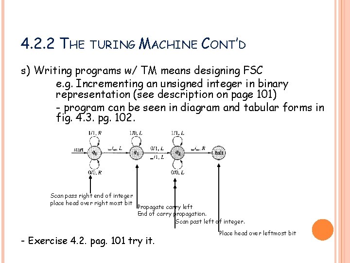
4. 2. 2 THE TURING MACHINE CONT’D s) Writing programs w/ TM means designing FSC e. g. Incrementing an unsigned integer in binary representation (see description on page 101) - program can be seen in diagram and tabular forms in fig. 4. 3. pg. 102. Scan pass right end of integer place head over right most bit Propagate carry left End of carry propagation. Scan past left of integer. - Exercise 4. 2. pag. 101 try it. Place head over leftmost bit

4. 2. 2 THE TURING MACHINE CONT’D S) Advantage of TM: - simplicity, uniformity - no need to make time and space complexity measures. (since there is only one type of instruction) - the time taken by a TM is the # steps taken by computation. - the space taken by a TM is the # distinct square tapes scanned during computation.

4. 2. 2 THE TURING MACHINE CONT’D S) DISADVANTAGE of TM: - it requires much time to carry out elementary operations (that a modern computer can execute in one instruction). S) SIMILARITIES between TM & Modern Computers a) Incrementing a number on a TM requires time proportional to the length of the number’s binary representation. Same is true for computers working with very large numbers. b) Accessing an arbitrary stored quantity cannot be done in constant time, either with TM or with modern computers.

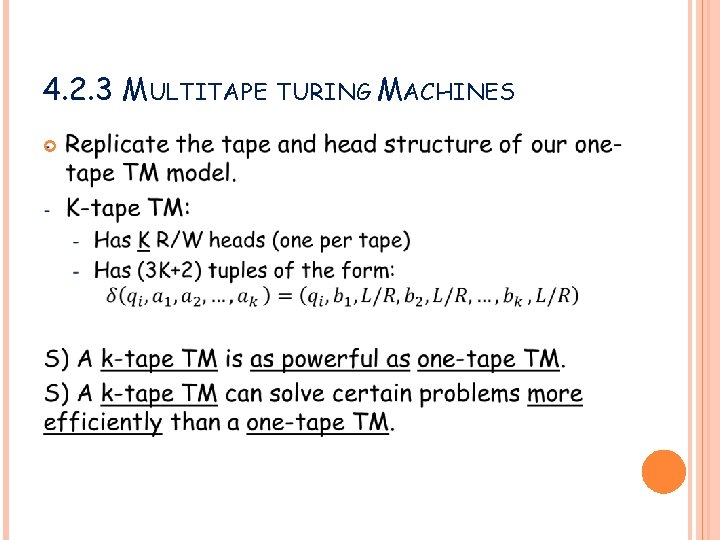
4. 2. 3 MULTITAPE TURING MACHINES

4. 2. 3 MULTITAPE TURING MACHINES CONT’D Exercise 4. 3 (page. 103): Verify that a two-tape Turing machine can recognize the language of palindromes over {0, 1} in time linear in the size of the input, while a one-tape TM requires quadratic time with the size of the input (in the worst case). Theorem 4. 1: A k-tape TM can be simulated by a standard one-tape machine at a cost of (at most) a quadratic increase in running time and a constant factor in space penalty. (See proof pages 103 -105. ) – simulating ktapes with single k-track tape.

4. 2. 3 MULTITAPE TURING MACHINES CONT’D Exercise 4. 3 (page. 103): Verify that a two-tape TM can recognize the language of palindromes over {0, 1} in time linear in the size of the input, while a one-tape TM requires a quadratic time with the size of the input (in the worst case). Theorem 4. 1: A k-tape TM can be simulated by a standard one-tape machine at a cost of (at most) a quadratic increase in running time and a constant factor in space penalty. (See proof pages 103 -105. ) – simulating k tapes with single k-track tape.

4. 2. 4 THE REGISTER MACHINE - RAM Ξ register machine (family) model (RM) - RM mimics modern computers Composition: - CPU - unbounded number of registers {each register can store an arbitrarily large integer} CPU carries out instructions on the registers, each of which can store an arbitrarily large integer. S) As in the case of TM, in RM the program is not stored in the memory that holds data => RM cannot be self-modifying => Any RM program can deal only with a fixed number of registers. -

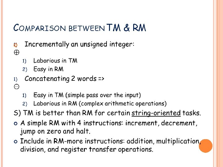
COMPARISON BETWEEN TM & RM

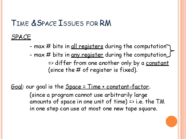
TIME &SPACE ISSUES FOR RM SPACE - max # bits in all registers during the computation - max # bits in any register during the computation => differ from one another only by a constant (since the # of register is fixed). Goal: our goal is the Space = Time + constant-factor. (since a program cannot use arbitrarily large amounts of space in one unit of time) => i. e. the TM in one step can use at most one new tape square.

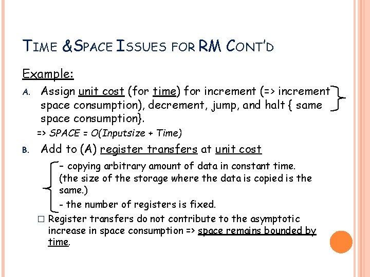
TIME &SPACE ISSUES FOR RM CONT’D Example: A. Assign unit cost (for time) for increment (=> increment space consumption), decrement, jump, and halt { same space consumption}. => SPACE = O(Inputsize + Time) B. Add to (A) register transfers at unit cost - copying arbitrary amount of data in constant time. (the size of the storage where the data is copied is the same. ) - the number of registers is fixed. � Register transfers do not contribute to the asymptotic increase in space consumption => space remains bounded by time.

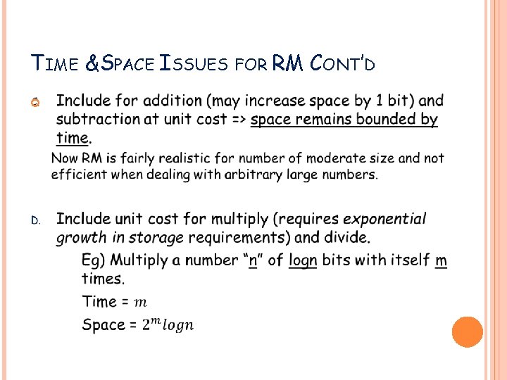
TIME &SPACE ISSUES FOR RM CONT’D

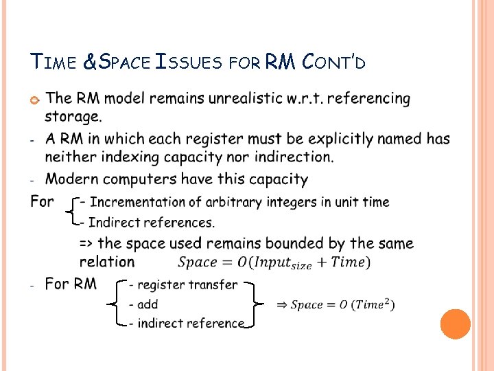
TIME &SPACE ISSUES FOR RM CONT’D

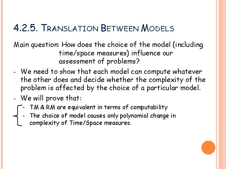
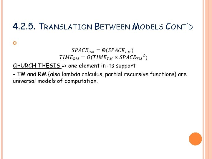
4. 2. 5. TRANSLATION BETWEEN MODELS Main question: How does the choice of the model (including time/space measures) influence our assessment of problems? - We need to show that each model can compute whatever the other does and decide whether the complexity of the problem is affected by the choice of a particular model. - We will prove that: TM & RM are equivalent in terms of computability - The choice of model causes only polynomial change in complexity of Time/Space measures. -

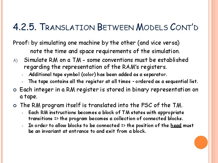
4. 2. 5. TRANSLATION BETWEEN MODELS CONT’D Proof: by simulating one machine by the other (and vice versa) note the time and space requirements of the simulation. Simulate RM on a TM - some conventions must be established regarding the representation of the RAM’s registers. A) - Additional tape symbol (color) has been added as a separator. The tape contains all the register at all times - ordered as a sequential list. Each integer in a RM register is stored in binary representation on a tape. The RM program itself is translated into the FSC of the TM. - Each RM instructions becomes a block of TM states with appropriate transitions => the program becomes a collection of connected blocks. In order to allow blocks to be connected => the position of the head must be an invariant at entrance to and exit from a block.

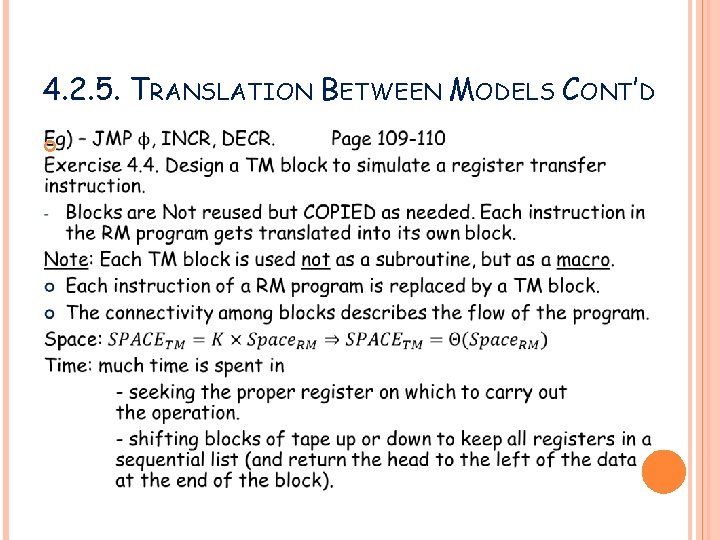
4. 2. 5. TRANSLATION BETWEEN MODELS CONT’D

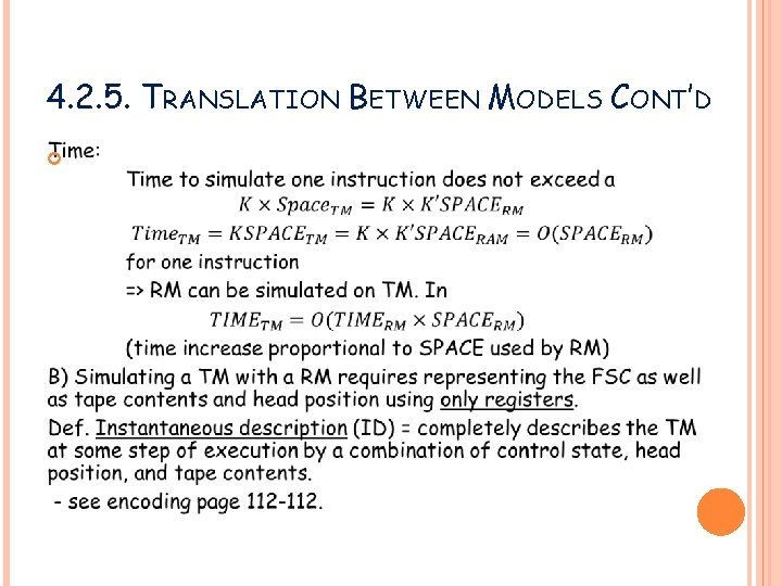
4. 2. 5. TRANSLATION BETWEEN MODELS CONT’D

4. 2. 5. TRANSLATION BETWEEN MODELS CONT’D