Modeling Computation Rosen ch 12 Modeling Computation We

Modeling Computation Rosen, ch. 12

Modeling Computation • We learned earlier the concept of an algorithm. – A description of a computational procedure. • Now, how can we model the computer itself, and what it is doing when it carries out an algorithm? – For this, we want to model the abstract process of computation itself.

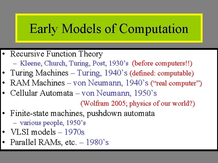
Early Models of Computation • Recursive Function Theory – Kleene, Church, Turing, Post, 1930’s (before computers!!) • Turing Machines – Turing, 1940’s (defined: computable) • RAM Machines – von Neumann, 1940’s (“real computer”) • Cellular Automata – von Neumann, 1950’s (Wolfram 2005; physics of our world? ) • Finite-state machines, pushdown automata – various people, 1950’s • VLSI models – 1970 s • Parallel RAMs, etc. – 1980’s

§ 12. 1 – Languages & Grammars • • Phrase-Structure Grammars Types of Phrase-Structure Grammars Derivation Trees Backus-Naur Form

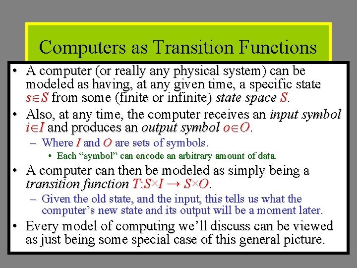
Computers as Transition Functions • A computer (or really any physical system) can be modeled as having, at any given time, a specific state s S from some (finite or infinite) state space S. • Also, at any time, the computer receives an input symbol i I and produces an output symbol o O. – Where I and O are sets of symbols. • Each “symbol” can encode an arbitrary amount of data. • A computer can then be modeled as simply being a transition function T: S×I → S×O. – Given the old state, and the input, this tells us what the computer’s new state and its output will be a moment later. • Every model of computing we’ll discuss can be viewed as just being some special case of this general picture.

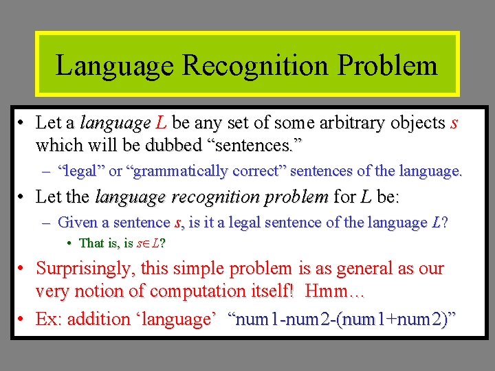
Language Recognition Problem • Let a language L be any set of some arbitrary objects s which will be dubbed “sentences. ” – “legal” or “grammatically correct” sentences of the language. • Let the language recognition problem for L be: – Given a sentence s, is it a legal sentence of the language L? • That is, is s L? • Surprisingly, this simple problem is as general as our very notion of computation itself! Hmm… • Ex: addition ‘language’ “num 1 -num 2 -(num 1+num 2)”

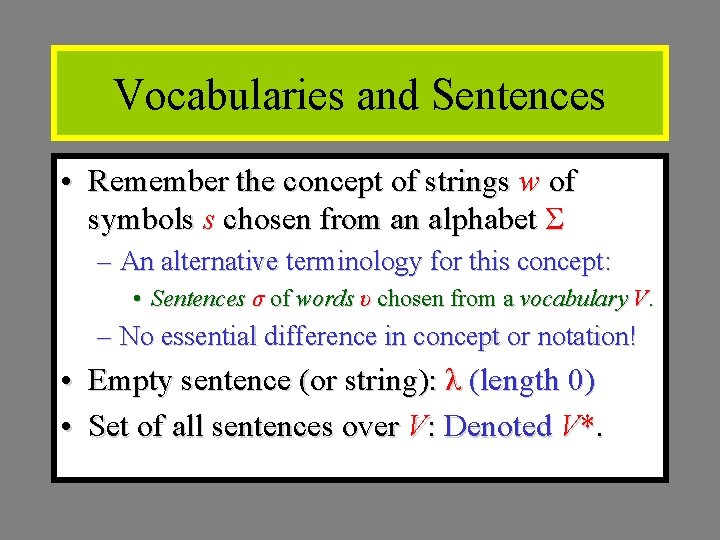
Vocabularies and Sentences • Remember the concept of strings w of symbols s chosen from an alphabet Σ – An alternative terminology for this concept: • Sentences σ of words υ chosen from a vocabulary V. – No essential difference in concept or notation! • Empty sentence (or string): λ (length 0) • Set of all sentences over V: Denoted V*.

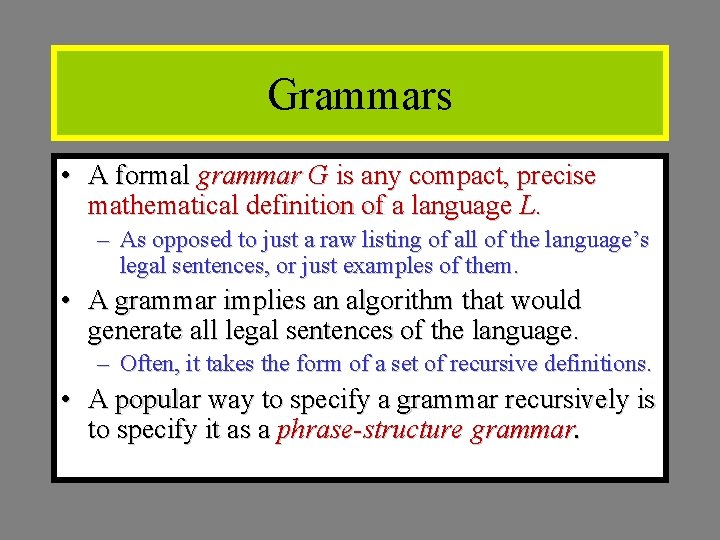
Grammars • A formal grammar G is any compact, precise mathematical definition of a language L. – As opposed to just a raw listing of all of the language’s legal sentences, or just examples of them. • A grammar implies an algorithm that would generate all legal sentences of the language. – Often, it takes the form of a set of recursive definitions. • A popular way to specify a grammar recursively is to specify it as a phrase-structure grammar.

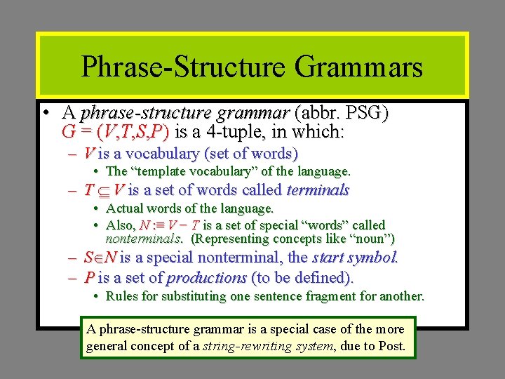
Phrase-Structure Grammars • A phrase-structure grammar (abbr. PSG) G = (V, T, S, P) is a 4 -tuple, in which: – V is a vocabulary (set of words) • The “template vocabulary” of the language. – T V is a set of words called terminals • • Actual words of the language. Also, N : ≡ V − T is a set of special “words” called nonterminals. (Representing concepts like “noun”) – S N is a special nonterminal, the start symbol. – P is a set of productions (to be defined). • Rules for substituting one sentence fragment for another. A phrase-structure grammar is a special case of the more general concept of a string-rewriting system, due to Post.

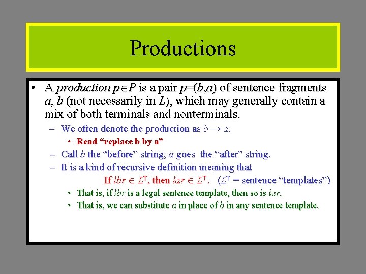
Productions • A production p P is a pair p=(b, a) of sentence fragments a, b (not necessarily in L), which may generally contain a mix of both terminals and nonterminals. – We often denote the production as b → a. • Read “replace b by a” – Call b the “before” string, a goes the “after” string. – It is a kind of recursive definition meaning that If lbr LT, then lar LT. (LT = sentence “templates”) • That is, if lbr is a legal sentence template, then so is lar. • That is, we can substitute a in place of b in any sentence template.

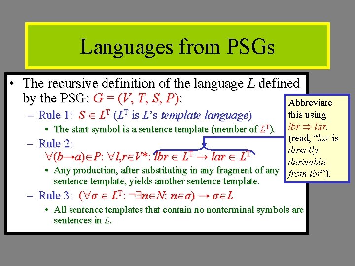
Languages from PSGs • The recursive definition of the language L defined by the PSG: G = (V, T, S, P): Abbreviate – Rule 1: S LT (LT is L’s template language) – this using • The start symbol is a sentence template (member of LT). lbr lar. (read, “lar is Rule 2: directly T T (b→a) P: l, r V*: lbr L → lar L derivable • Any production, after substituting in any fragment of any from lbr”). sentence template, yields another sentence template. – Rule 3: ( σ LT: ¬ n N: n σ) → σ L • All sentence templates that contain no nonterminal symbols are sentences in L.

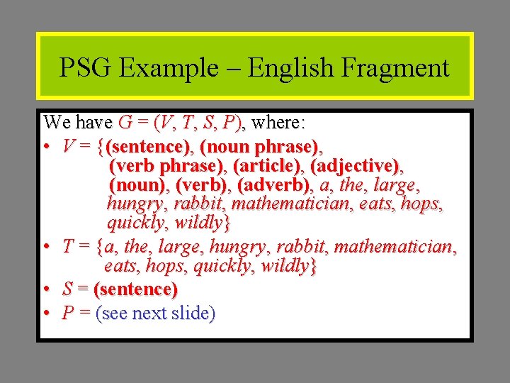
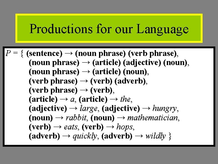
PSG Example – English Fragment We have G = (V, T, S, P), where: • V = {(sentence), (noun phrase), (verb phrase), (article), (adjective), (noun), (verb), (adverb), a, the, large, hungry, rabbit, mathematician, eats, hops, quickly, wildly} • T = {a, the, large, hungry, rabbit, mathematician, eats, hops, quickly, wildly} • S = (sentence) • P = (see next slide)

Productions for our Language P = { (sentence) → (noun phrase) (verb phrase), (noun phrase) → (article) (adjective) (noun), (noun phrase) → (article) (noun), (verb phrase) → (verb) (adverb), (verb phrase) → (verb), (article) → a, (article) → the, (adjective) → large, (adjective) → hungry, (noun) → rabbit, (noun) → mathematician, (verb) → eats, (verb) → hops, (adverb) → quickly, (adverb) → wildly }

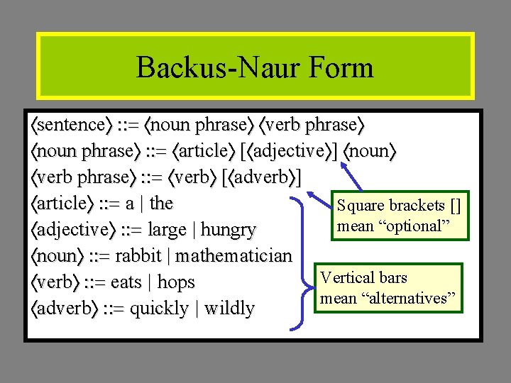
Backus-Naur Form sentence : : = noun phrase verb phrase noun phrase : : = article [ adjective ] noun verb phrase : : = verb [ adverb ] article : : = a | the Square brackets [] mean “optional” adjective : : = large | hungry noun : : = rabbit | mathematician Vertical bars verb : : = eats | hops mean “alternatives” adverb : : = quickly | wildly

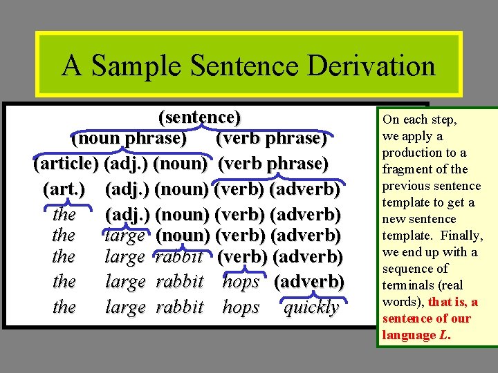
A Sample Sentence Derivation (sentence) (noun phrase) (verb phrase) (article) (adj. ) (noun) (verb phrase) (art. ) (adj. ) (noun) (verb) (adverb) the (adj. ) (noun) (verb) (adverb) the large rabbit (verb) (adverb) the large rabbit hops (adverb) the large rabbit hops quickly On each step, we apply a production to a fragment of the previous sentence template to get a new sentence template. Finally, we end up with a sequence of terminals (real words), that is, a sentence of our language L.

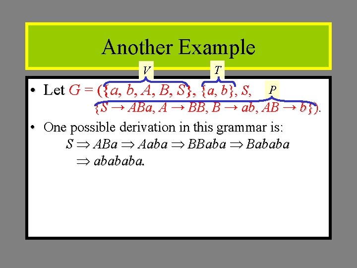
Another Example V T • Let G = ({a, b, A, B, S}, {a, b}, S, P {S → ABa, A → BB, B → ab, AB → b}). • One possible derivation in this grammar is: S ABa Aaba BBaba Bababa abababa.

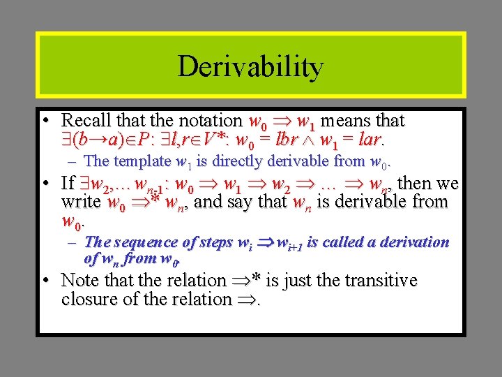
Derivability • Recall that the notation w 0 w 1 means that (b→a) P: l, r V*: w 0 = lbr w 1 = lar. – The template w 1 is directly derivable from w 0. • If w 2, …wn-1: w 0 w 1 w 2 … wn, then we write w 0 * wn, and say that wn is derivable from w 0. – The sequence of steps wi wi+1 is called a derivation of wn from w 0. • Note that the relation * is just the transitive closure of the relation .

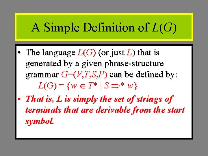
A Simple Definition of L(G) • The language L(G) (or just L) that is generated by a given phrase-structure grammar G=(V, T, S, P) can be defined by: L(G) = {w T* | S * w} • That is, L is simply the set of strings of terminals that are derivable from the start symbol.

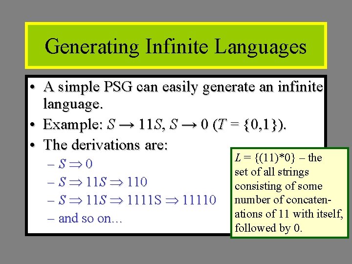
Generating Infinite Languages • A simple PSG can easily generate an infinite language. • Example: S → 11 S, S → 0 (T = {0, 1}). • The derivations are: – S 0 – S 11 S 1111 S 11110 – and so on… L = {(11)*0} – the set of all strings consisting of some number of concatenations of 11 with itself, followed by 0.

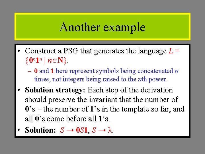
Another example • Construct a PSG that generates the language L = {0 n 1 n | n N}. – 0 and 1 here represent symbols being concatenated n times, not integers being raised to the nth power. • Solution strategy: Each step of the derivation should preserve the invariant that the number of 0’s = the number of 1’s in the template so far, and all 0’s come before all 1’s. • Solution: S → 0 S 1, S → λ.

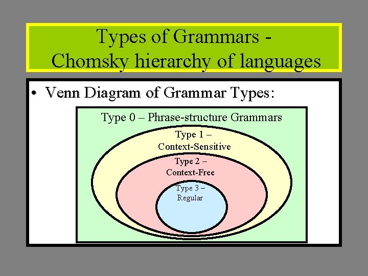
Types of Grammars Chomsky hierarchy of languages • Venn Diagram of Grammar Types: Type 0 – Phrase-structure Grammars Type 1 – Context-Sensitive Type 2 – Context-Free Type 3 – Regular

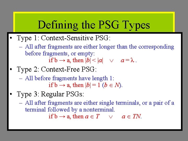
Defining the PSG Types • Type 1: Context-Sensitive PSG: – All after fragments are either longer than the corresponding before fragments, or empty: if b → a, then |b| < |a| a = λ. • Type 2: Context-Free PSG: – All before fragments have length 1: if b → a, then |b| = 1 (b N). • Type 3: Regular PSGs: – All after fragments are either single terminals, or a pair of a terminal followed by a nonterminal. if b → a, then a T a TN.

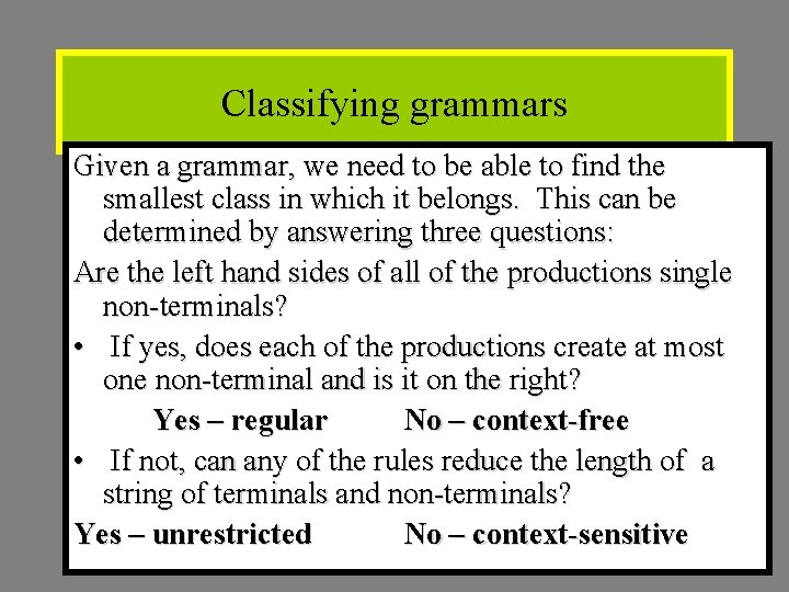
Classifying grammars Given a grammar, we need to be able to find the smallest class in which it belongs. This can be determined by answering three questions: Are the left hand sides of all of the productions single non-terminals? • If yes, does each of the productions create at most one non-terminal and is it on the right? Yes – regular No – context-free • If not, can any of the rules reduce the length of a string of terminals and non-terminals? Yes – unrestricted No – context-sensitive

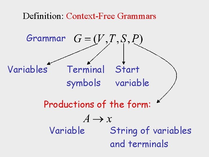
Definition: Context-Free Grammars Grammar Variables Terminal symbols Start variable Productions of the form: Variable String of variables and terminals

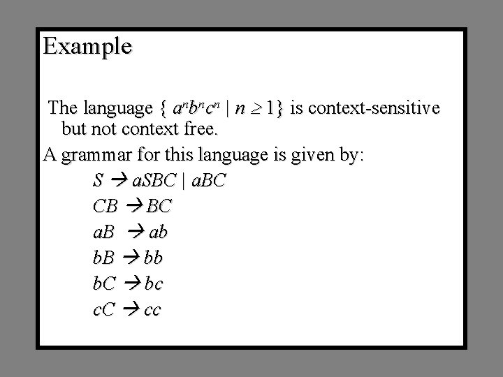
Example The language { anbncn | n 1} is context-sensitive but not context free. A grammar for this language is given by: S a. SBC | a. BC CB BC a. B ab b. B bb b. C bc c. C cc

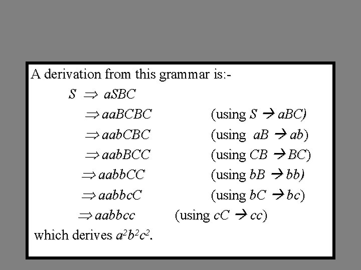
A derivation from this grammar is: S a. SBC aa. BCBC (using S a. BC) aab. CBC (using a. B ab) aab. BCC (using CB BC) aabb. CC (using b. B bb) aabbc. C (using b. C bc) aabbcc (using c. C cc) which derives a 2 b 2 c 2.