TOPICS IN DEEP LEARNING Computation Graphs A computation

TOPICS IN DEEP LEARNING

Computation Graphs ØA computation graph is a way to represent computation in software ØIt is a directed acyclic graph (DAG) in which: ØNodes – corresponds to variables, constants or mathematical operations ØEdges – corresponds to the flow of intermediary values ØNo need for ‘()’ in computation graphs, calculation is defined by topological sort ØUsed to calculate both function values and gradients

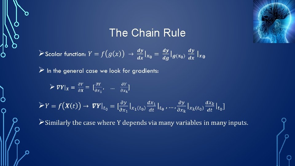
The Chain Rule •

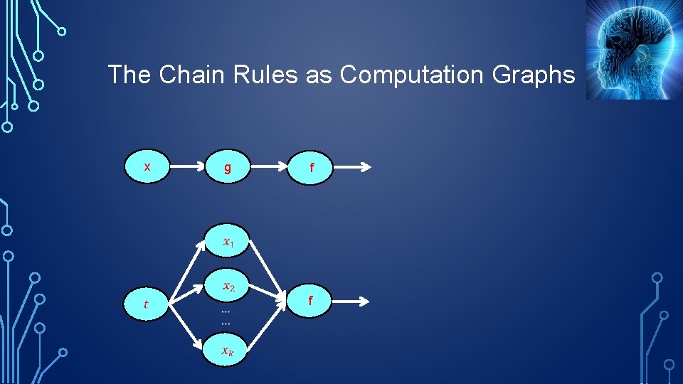
The Chain Rules as Computation Graphs x g f f

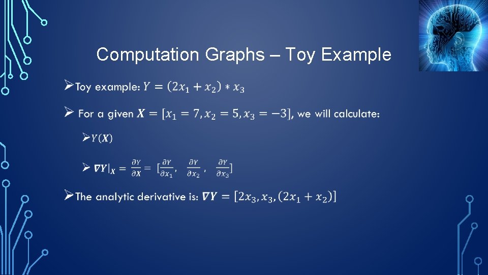
Computation Graphs – Toy Example •

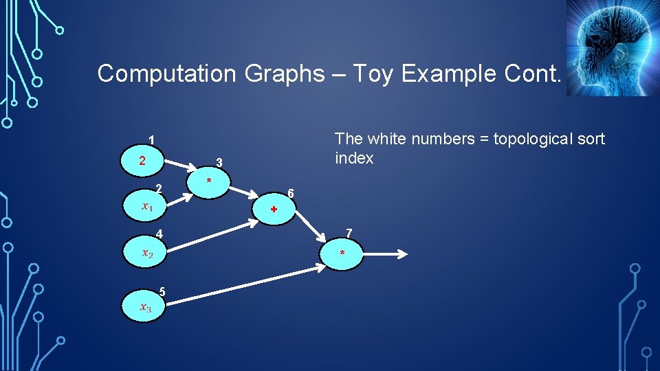
Computation Graphs – Toy Example Cont. The white numbers = topological sort index 1 2 3 2 * 6 + 7 4 * 5

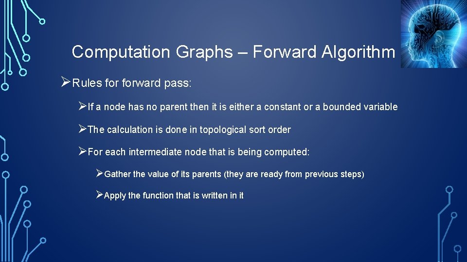
Computation Graphs – Forward Algorithm ØRules forward pass: ØIf a node has no parent then it is either a constant or a bounded variable ØThe calculation is done in topological sort order ØFor each intermediate node that is being computed: ØGather the value of its parents (they are ready from previous steps) ØApply the function that is written in it

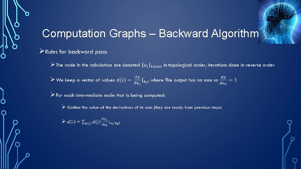
Computation Graphs – Backward Algorithm •

Computation Graphs – Software Packages ØThe most commonly used software packages are: ØTensor. Flow – Google (similar to Theano) ØCaffe 2 – Facebook (has predefined models) ØPy. Torch – mostly used by researchers ØMXNet – Amazon a new player in the court ØWrappers - Keras

Software Packages – Main Features ØDefinition of computation graph (static / dynamic graphs): ØFunction evaluation ØAutomatic derivative ØAutomatic training - support for mini batchs ØSupport GPU’s / cloud computing ØPre-defined layers/ Pre-trained models

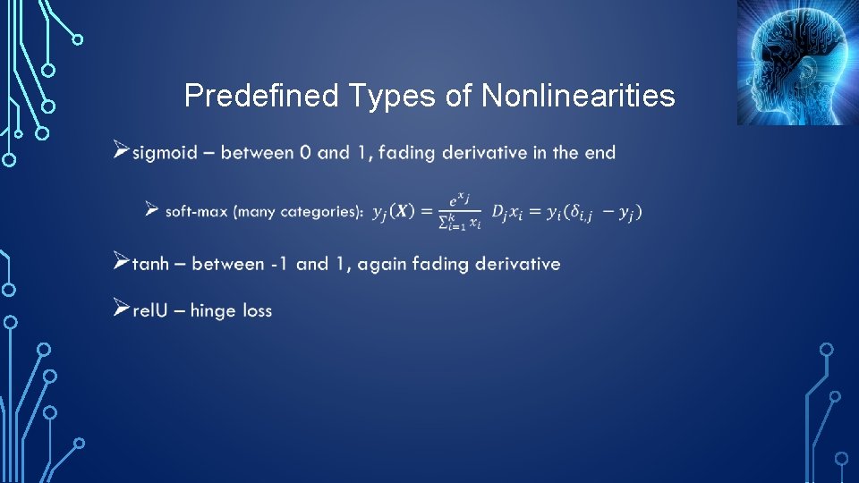
Predefined Types of Nonlinearities •

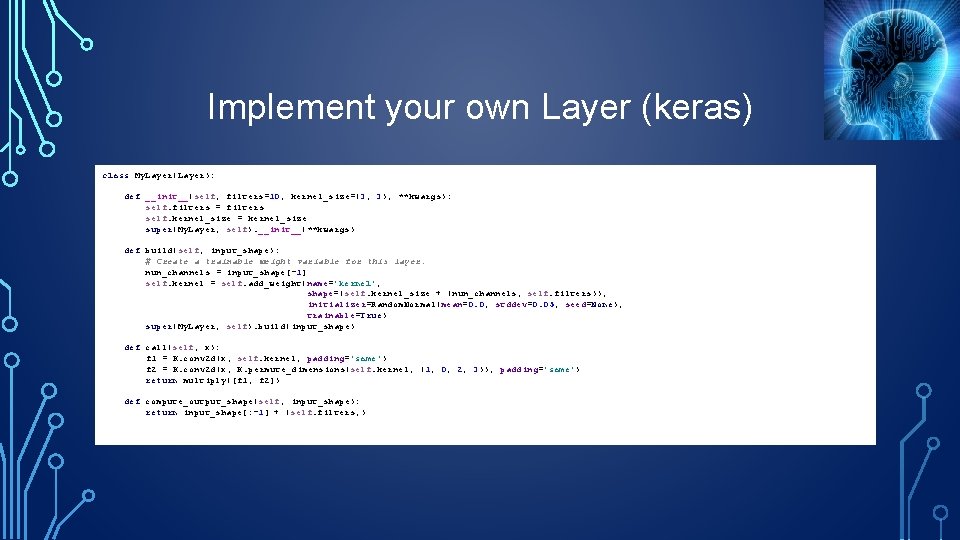
Implement your own Layer (keras) class My. Layer(Layer): def __init__(self, filters=10, kernel_size=(3, 3), **kwargs): self. filters = filters self. kernel_size = kernel_size super(My. Layer, self). __init__(**kwargs) def build(self, input_shape): # Create a trainable weight variable for this layer. nun_channels = input_shape[-1] self. kernel = self. add_weight(name='kernel', shape=(self. kernel_size + (nun_channels, self. filters)), initializer=Random. Normal(mean=0. 0, stddev=0. 05, seed=None), trainable=True) super(My. Layer, self). build(input_shape) def call(self, x): f 1 = K. conv 2 d(x, self. kernel, padding='same') f 2 = K. conv 2 d(x, K. permute_dimensions(self. kernel, (1, 0, 2, 3)), padding='same') return multiply([f 1, f 2]) def compute_output_shape(self, input_shape): return input_shape[: -1] + (self. filters, )

Predefined Types of Layers ØFully connected (Dense) ØAll inputs connected to all outputs ØUsed as classifier for example ØBatchnorm – normalize the outputs, not very fashionable nowadays ØDropout – used for regulatization only during training ØDuring the train randomly drop p of the vertices and scale all the others

Predefined Types of Layers – Cont. ØConv 2 d – perform convolution on the image Our subject on the next slides ØEmbedding – calculate a mapping of objects (e. g. , word) to vector representation The subject right after it ØLSTM – used for sequences of unknown size, recurrent transformations (if time permits I will talk about it)

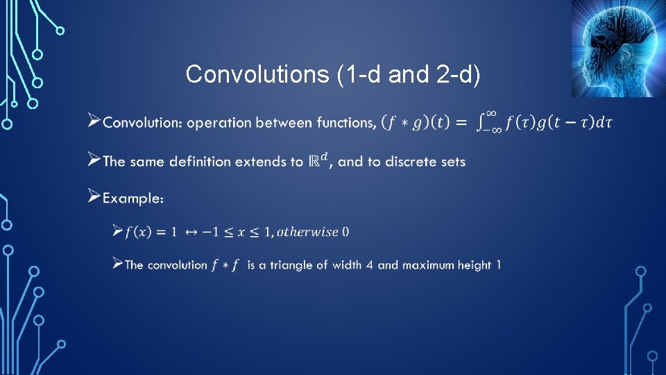
Convolutions (1 -d and 2 -d) •

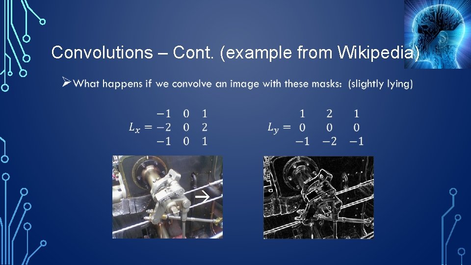
Convolutions – Cont. (example from Wikipedia) •

Convolution in Image Processing ØA very useful tool for edge detection, smoothing, sharpening and other operations. ØBut all these are manual made filters. ØCan we let the system learn the filters ? ØWhat happens if we run the filters one on top of the other ? ØCan we match a filter to detect certain shapes ?

From Convolutions to Convoltion-NN ØConvolution is linear, so running two filters consecutively is equivalent to have a different filter applied once. So some non-linearity is required. ØA convolution neural network does exactly what we have asked in the previous slide: ØIt learns a set of filters ØIt uses non-linearity to get a more complex results ØThe layers matches themselves to the object we want to learn

The Challenge of Image Classification - Image. Net ØImage. Net is a dataset of labeled images taken from the internet ØOver 14 M color images: 224 X 3 ØOver 20 K categories (nested) ØThe challenge (approximately 1 K categories) was announced at 2010 ØThe error was > 25% before 2012 ØIn 2012 Conv. Net got 16% error !!!

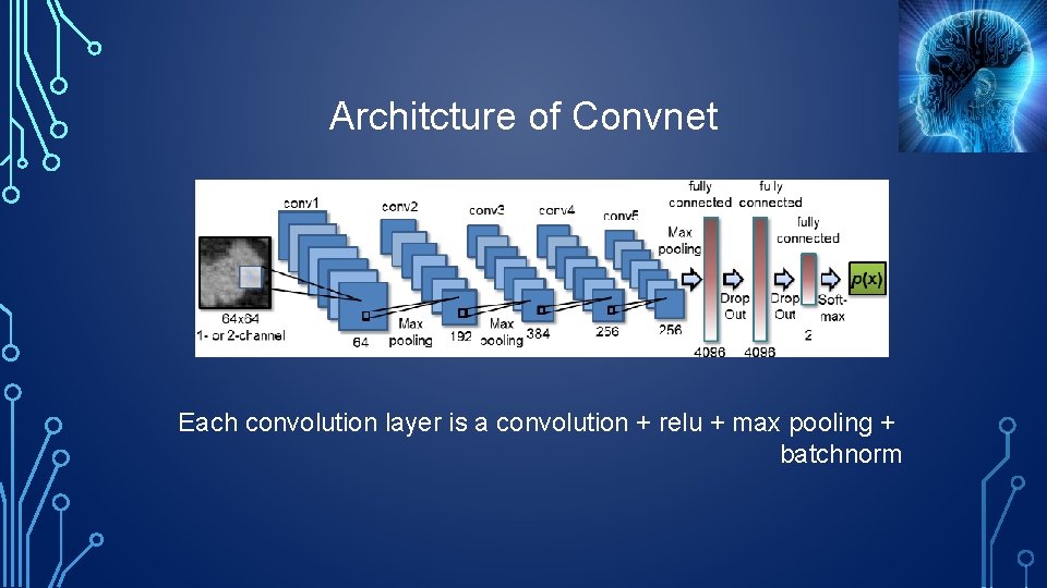
Architcture of Convnet Each convolution layer is a convolution + relu + max pooling + batchnorm

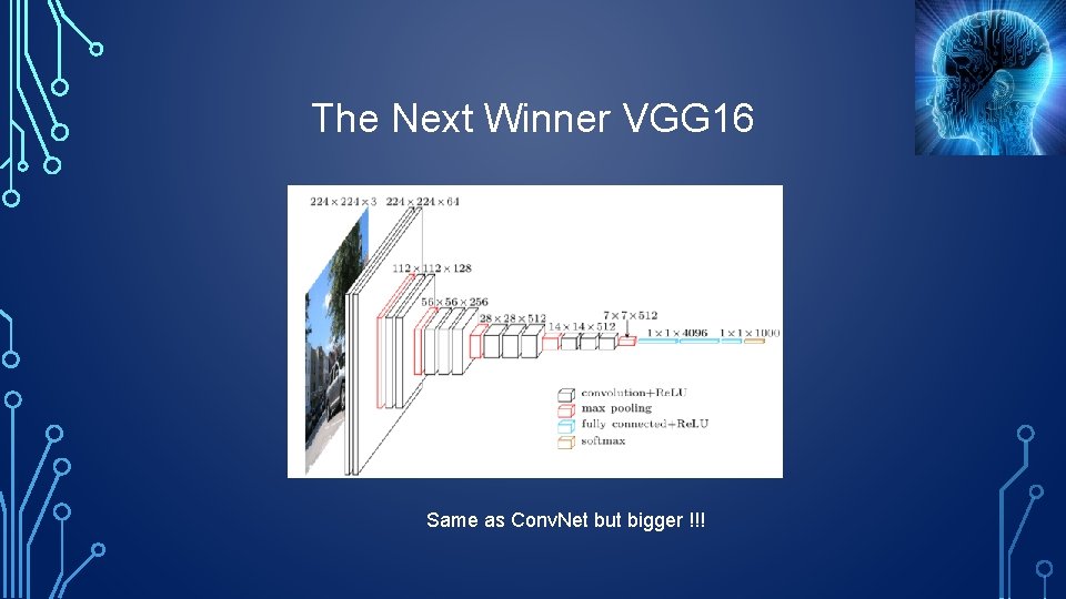
The Next Winner VGG 16 Same as Conv. Net but bigger !!!

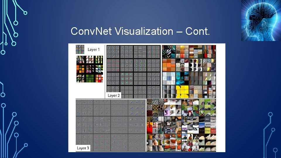
Conv. Net Visualization ØCan we visualize what the network have learned ? ØFor first layer the results are linear filters and they can easily be visualized ØWhat about the next layers ? ØWhy is it interesting ? ØThe next slides are taken from Zeiler and Fergus 2013, “Visualizing and Understanding Convolutional Networks”

Conv. Net Visualization – Cont.

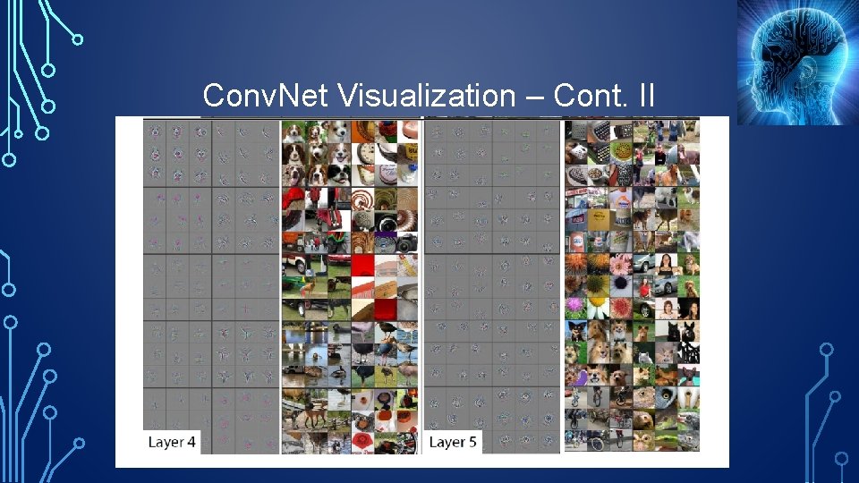
Conv. Net Visualization – Cont. II

Conv. Net Visualization – Cont. III ØThe secret behind these images is the deconv layer: ØRevert the maxpooling ØThe relu is preserved if active ØThe filter needs to be transposed (I won’t explain why) ØThis layer is used in other reconstruction problems ØAnother secret is of course to select the right images !!!

resnet – The New Architecture Type ØThe 2016 winner has defeated everyone in all criteria – resnet

Word 2 Vec ØIn language problems we may want to use words as features ØThe obvious solution people are using for over 20 years is to take each word as an indicator (with some enhancements) ØThis representation loses all notion of proximity ØWe would like to map a Vocabulary to a vector space in a way that preserves semantic (and syntactic) relations

Word 2 Vec – Cont. Ø“You shall know a word by the company that it keeps” (Firth 1957) ØHow can we exploit this distributional similarity to study a representation ? ØWe define a vector for each word (distributed representation) ØThese vectors should be such that you can predict neighboring words from them ØWord 2 Vec is an algorithm that finds this vector representation

Word 2 Vec – Cont. II •

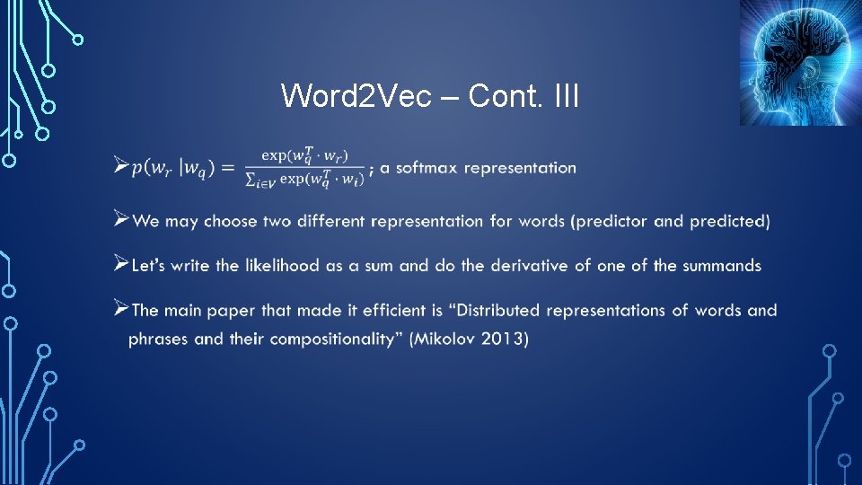
Word 2 Vec – Cont. III •

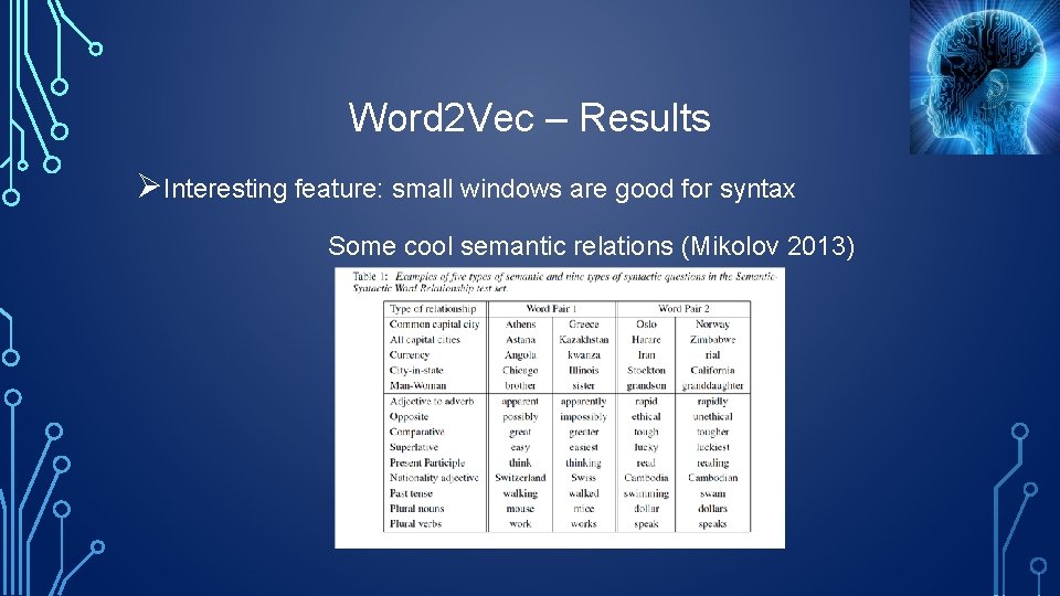
Word 2 Vec – Results ØInteresting feature: small windows are good for syntax Some cool semantic relations (Mikolov 2013)

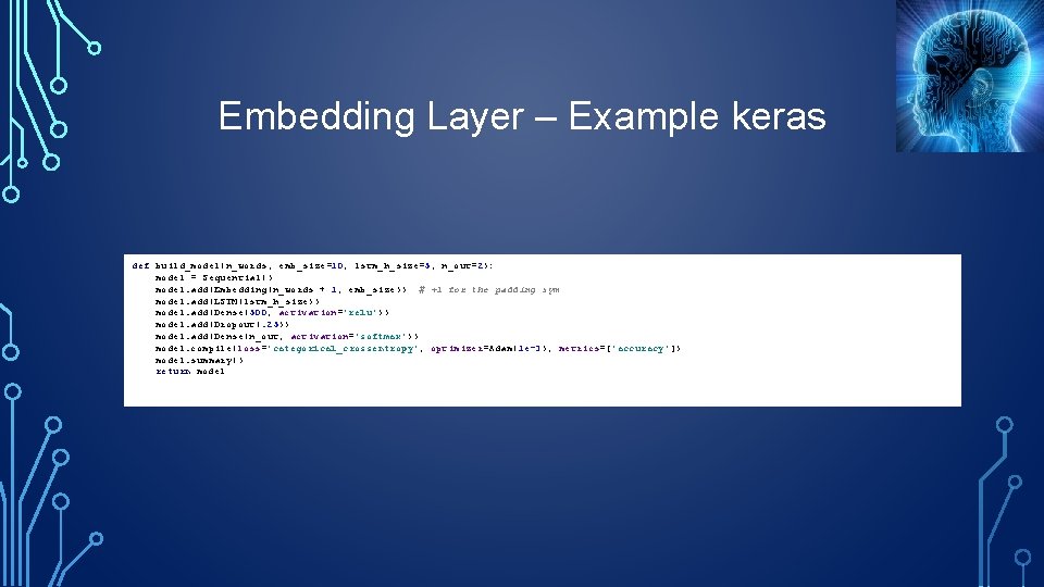
Embedding Layer ØIn Word 2 Vec we learned the representation solving a classification problem ØThis problem was unsupervised since we learned proximity ØIn Embedding layer we also learn proximity, for example as a step in a supervised learning problem ØIt is similar to using principal components as features in a regression

Embedding Layer – Example keras def build_model(n_words, emb_size=10, lstm_h_size=5, n_out=2): model = Sequential() model. add(Embedding(n_words + 1, emb_size)) # +1 for the padding sym model. add(LSTM(lstm_h_size)) model. add(Dense(500, activation='relu')) model. add(Dropout(. 25)) model. add(Dense(n_out, activation='softmax')) model. compile(loss='categorical_crossentropy', optimizer=Adam(1 e-3), metrics=['accuracy']) model. summary() return model

Generative Adversarial Network ØGenerative models - find the probabilistic process that generates the data ØCan be done parametrically using approximation to the likelihood ØGAN changed the focus and since then this is by far the most used model ØThe generating distribution is not kept in an explicit form ØThe original paper is: “Generative Adversarial Nets” (Goodfellow 2014)

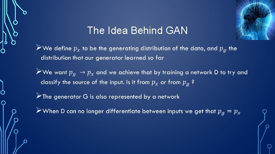
The Idea Behind GAN •