Modeling Computation EECS 1019 Discrete Math for CS

Modeling Computation EECS 1019: Discrete Math for CS Prof. Andy Mirzaian © 2019 Mc. Graw-Hill Education. All rights reserved. Authorized only for instructor use in the classroom. No reproduction or further distribution permitted without the prior written consent of Mc. Graw-Hill Education.

Chapter Summary Languages and Grammars Finite-State Machines with Output Finite-State Machines with No Output Language Recognition Turing Machines 2 © 2019 Mc. Graw-Hill Education

Languages and Grammars Section 13. 1 3 © 2019 Mc. Graw-Hill Education

Section Summary 1 Phrase-Structure Grammars Types of Phrase-Structure Grammars Derivation Trees Backus-Naur Form 4 © 2019 Mc. Graw-Hill Education

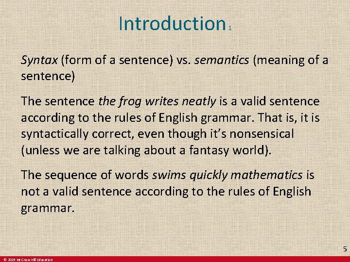
Introduction 1 Syntax (form of a sentence) vs. semantics (meaning of a sentence) The sentence the frog writes neatly is a valid sentence according to the rules of English grammar. That is, it is syntactically correct, even though it’s nonsensical (unless we are talking about a fantasy world). The sequence of words swims quickly mathematics is not a valid sentence according to the rules of English grammar. 5 © 2019 Mc. Graw-Hill Education

Grammars The rules that specify the syntactically correct sentences of a natural language such as English are complex. Instead of studying natural languages, we can define formal languages that have well-defined rules of syntax. These rules of syntax are important both in linguistics (the study of natural languages) and in the study of programming languages. 6 © 2019 Mc. Graw-Hill Education

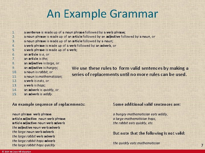
An Example Grammar 1. 2. 3. 4. 5. 6. 7. 8. 9. 10. 11. 12. 13. 14. 15. a sentence is made up of a noun phrase followed by a verb phrase; a noun phrase is made up of an article followed by an adjective followed by a noun, or a noun phrase is made up of an article followed by a noun; a verb phrase is made up of a verb followed by an adverb, or a verb phrase is made up of a verb; an article is a, or an article is the; an adjective is large, or an adjective is hungry; We use these rules to form valid sentences by making a a noun is rabbit, or series of replacements until no more rules can be used. a noun is mathematician; a verb is eats, or a verb is hops; an adverb is quickly, or an adverb is wildly. An example sequence of replacements: Some additional valid sentences are: noun phrase verb phrase article adjective noun verb adverb the large rabbit verb adverb the large rabbit hops quickly a hungry mathematician eats wildly, a large mathematician hops, the rabbit eats quickly, etc. © 2019 Mc. Graw-Hill Education But note that the following is not valid: the quickly eats mathematician 7

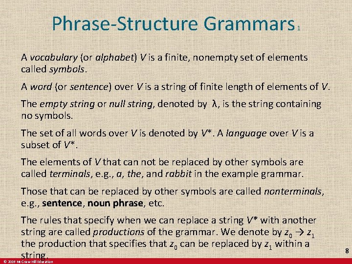
Phrase-Structure Grammars 1 A vocabulary (or alphabet) V is a finite, nonempty set of elements called symbols. A word (or sentence) over V is a string of finite length of elements of V. The empty string or null string, denoted by λ, is the string containing no symbols. The set of all words over V is denoted by V*. A language over V is a subset of V*. The elements of V that can not be replaced by other symbols are called terminals, e. g. , a, the, and rabbit in the example grammar. Those that can be replaced by other symbols are called nonterminals, e. g. , sentence, noun phrase, etc. The rules that specify when we can replace a string V* with another string are called productions of the grammar. We denote by z 0 → z 1 the production that specifies that z 0 can be replaced by z 1 within a string. © 2019 Mc. Graw-Hill Education 8

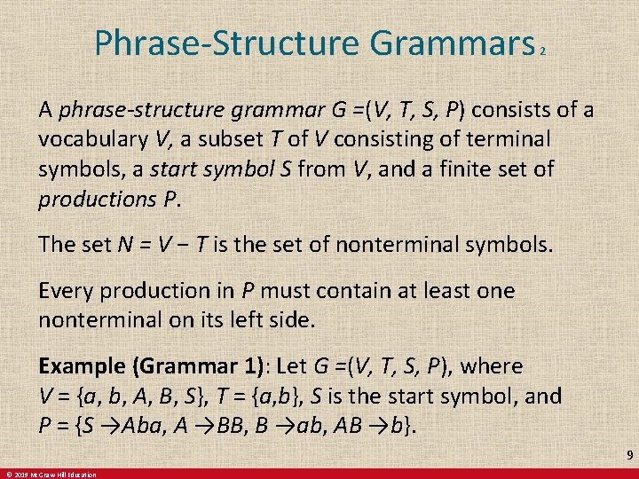
Phrase-Structure Grammars 2 A phrase-structure grammar G =(V, T, S, P) consists of a vocabulary V, a subset T of V consisting of terminal symbols, a start symbol S from V, and a finite set of productions P. The set N = V − T is the set of nonterminal symbols. Every production in P must contain at least one nonterminal on its left side. Example (Grammar 1): Let G =(V, T, S, P), where V = {a, b, A, B, S}, T = {a, b}, S is the start symbol, and P = {S →Aba, A →BB, B →ab, AB →b}. 9 © 2019 Mc. Graw-Hill Education

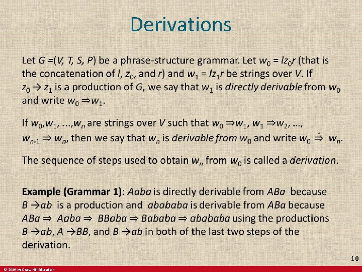
Derivations 10 © 2019 Mc. Graw-Hill Education

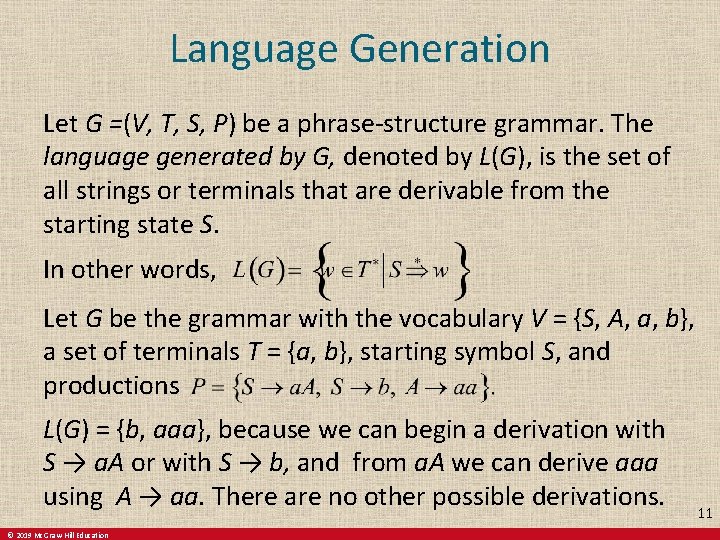
Language Generation Let G =(V, T, S, P) be a phrase-structure grammar. The language generated by G, denoted by L(G), is the set of all strings or terminals that are derivable from the starting state S. In other words, Let G be the grammar with the vocabulary V = {S, A, a, b}, a set of terminals T = {a, b}, starting symbol S, and productions L(G) = {b, aaa}, because we can begin a derivation with S → a. A or with S → b, and from a. A we can derive aaa using A → aa. There are no other possible derivations. © 2019 Mc. Graw-Hill Education 11

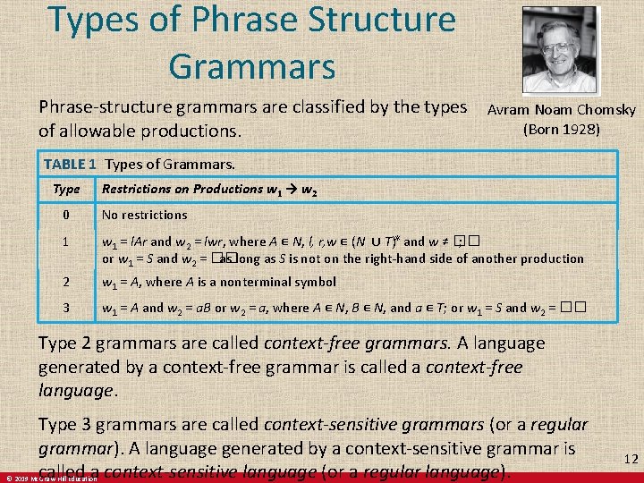
Types of Phrase Structure Grammars Phrase-structure grammars are classified by the types Avram Noam Chomsky (Born 1928) of allowable productions. TABLE 1 Types of Grammars. Type Restrictions on Productions w 1 → w 2 0 No restrictions 1 w 1 = l. Ar and w 2 = lwr, where A ∊ N, l, r, w ∊ (N ∪ T)∗ and w ≠ �� ; or w 1 = S and w 2 = �� as long as S is not on the right-hand side of another production 2 w 1 = A, where A is a nonterminal symbol 3 w 1 = A and w 2 = a. B or w 2 = a, where A ∊ N, B ∊ N, and a ∊ T; or w 1 = S and w 2 = �� Type 2 grammars are called context-free grammars. A language generated by a context-free grammar is called a context-free language. Type 3 grammars are called context-sensitive grammars (or a regular grammar). A language generated by a context-sensitive grammar is called a context-sensitive language (or a regular language). © 2019 Mc. Graw-Hill Education 12

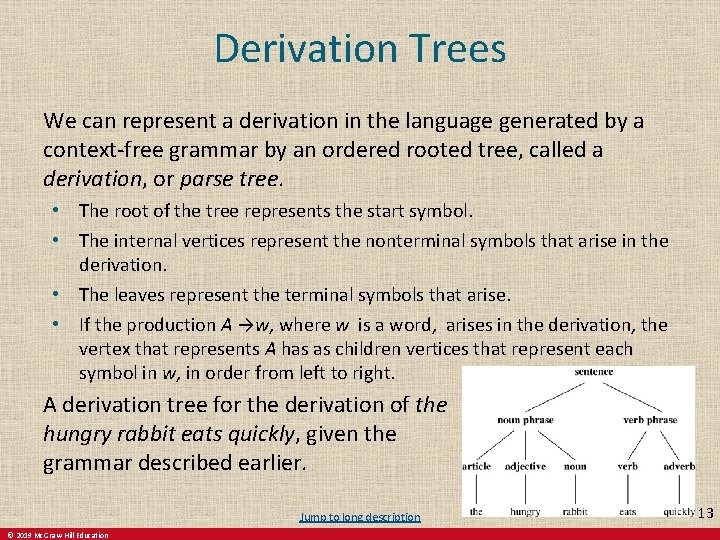
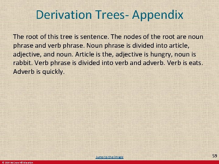
Derivation Trees We can represent a derivation in the language generated by a context-free grammar by an ordered rooted tree, called a derivation, or parse tree. • The root of the tree represents the start symbol. • The internal vertices represent the nonterminal symbols that arise in the derivation. • The leaves represent the terminal symbols that arise. • If the production A →w, where w is a word, arises in the derivation, the vertex that represents A has as children vertices that represent each symbol in w, in order from left to right. A derivation tree for the derivation of the hungry rabbit eats quickly, given the grammar described earlier. Jump to long description © 2019 Mc. Graw-Hill Education 13

Backus-Naur Form John Backus (1924 -2007) Peter Naur (Born 1928) Backus-Naur form (BNF) is sometimes used to specify a type 2 grammar. It is often used to specify the syntactic rules of computer languages. The productions of a type 2 grammar have a single nonterminal symbol on their left-hand side. All the productions with the same nonterminal symbol on the left-hand side are combined into one statement using the symbol : : = instead of →. Additionally, all nonterminal symbols are enclosed in brackets (�� ), and the right-hand side of productions are separated by bars. For example, the productions A →Aa, A →a, and A →AB are written as © 2019 Mc. Graw-Hill Education 14

BNF and ALGOL 60 In the programming language ALGOL 60 an identifier consists of a string of alphanumeric characters and must begin with a letter. The BNF description of allowable identifiers is: x 99 a is a valid identifier since the first rule can be used to replace �identifier� by �identifier�� letter� , the second rule to obtain �identifier�a, the first rule twice to obtain �identifier�� digit� a, the third rule twice to obtain �identifier� 99 a, the first rule to obtain �letter� 99 a, and finally the second rule to obtain x 99 a. © 2019 Mc. Graw-Hill Education 15

Finite-State Machines with Output Section 13. 2 16 © 2019 Mc. Graw-Hill Education

Section Summary 2 Finite-State Machines (FSMs) with Outputs Types of Finite-State Machines with Outputs (not currently included in overheads) 17 © 2019 Mc. Graw-Hill Education

Introduction 2 Many kinds of machines, including computers, can be modeled using a structure called a finite-state machine (or finite automaton). A finite-state machine consists of a finite set of states, a designated start state, an input alphabet, and a transition function that assigns a next state to every (state, input) pair As we will see in Sections 13. 2 − 13. 4, some types of finite-state machines produce output, while for other types of finite-state machines that do not produce output some states are designated as accepting states. Finite-state machines are used in many diverse applications, including spell-checking programs, grammar checking, indexing, searching large bodies of text, speech recognition, XML, HTML, and network protocols 18 © 2019 Mc. Graw-Hill Education

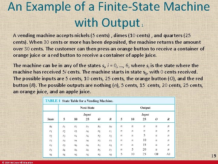
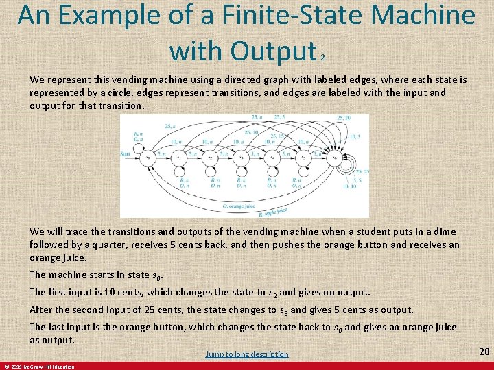
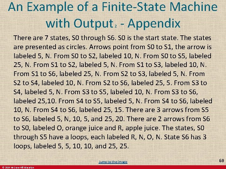
An Example of a Finite-State Machine with Output 1 A vending machine accepts nickels (5 cents) , dimes (10 cents) , and quarters (25 cents). When 30 cents or more has been deposited, the machine returns the amount over 30 cents. The customer can then press an orange button to receive a container of orange juice or a red button to receive a container of apple juice. The machine can be in any of the states si, i = 0, …, 6, where si is the state where the machine has received 5 i cents. The machine starts in state s 0, with 0 cents received. The possible inputs are 5 cents, 10 cents, 25 cents, the orange button (O), and the red button (R). The possible outputs are nothing (n), 5 cents, 15 cents, 20 cents, 25 cents, an orange juice, and an apple juice. 19 © 2019 Mc. Graw-Hill Education

An Example of a Finite-State Machine with Output 2 We represent this vending machine using a directed graph with labeled edges, where each state is represented by a circle, edges represent transitions, and edges are labeled with the input and output for that transition. We will trace the transitions and outputs of the vending machine when a student puts in a dime followed by a quarter, receives 5 cents back, and then pushes the orange button and receives an orange juice. The machine starts in state s 0. The first input is 10 cents, which changes the state to s 2 and gives no output. After the second input of 25 cents, the state changes to s 6 and gives 5 cents as output. The last input is the orange button, which changes the state back to s 0 and gives an orange juice as output. Jump to long description © 2019 Mc. Graw-Hill Education 20

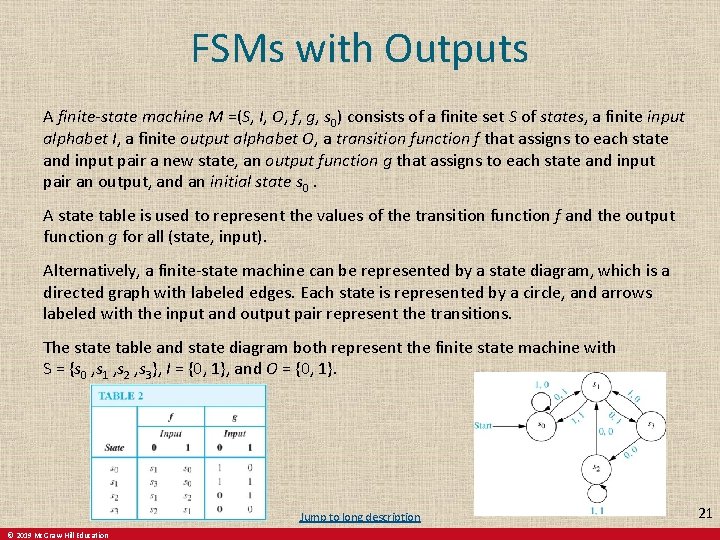
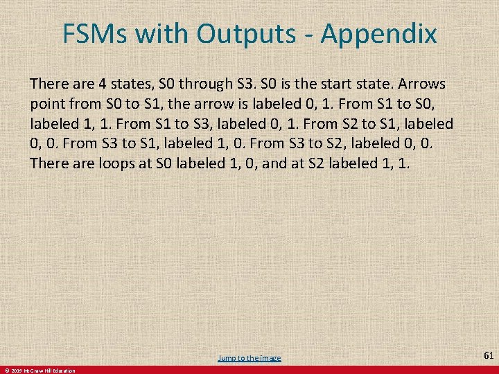
FSMs with Outputs A finite-state machine M =(S, I, O, f, g, s 0) consists of a finite set S of states, a finite input alphabet I, a finite output alphabet O, a transition function f that assigns to each state and input pair a new state, an output function g that assigns to each state and input pair an output, and an initial state s 0. A state table is used to represent the values of the transition function f and the output function g for all (state, input). Alternatively, a finite-state machine can be represented by a state diagram, which is a directed graph with labeled edges. Each state is represented by a circle, and arrows labeled with the input and output pair represent the transitions. The state table and state diagram both represent the finite state machine with S = {s 0 , s 1 , s 2 , s 3}, I = {0, 1}, and O = {0, 1}. Jump to long description © 2019 Mc. Graw-Hill Education 21

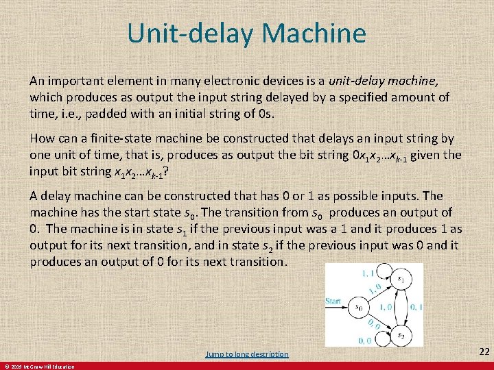
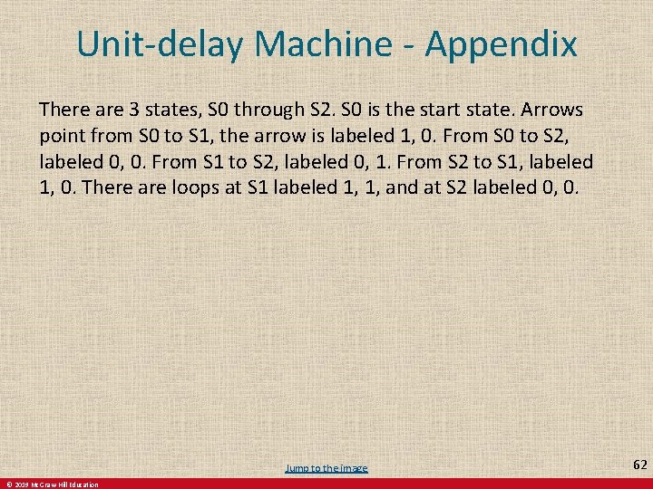
Unit-delay Machine An important element in many electronic devices is a unit-delay machine, which produces as output the input string delayed by a specified amount of time, i. e. , padded with an initial string of 0 s. How can a finite-state machine be constructed that delays an input string by one unit of time, that is, produces as output the bit string 0 x 1 x 2…xk-1 given the input bit string x 1 x 2…xk-1? A delay machine can be constructed that has 0 or 1 as possible inputs. The machine has the start state s 0. The transition from s 0 produces an output of 0. The machine is in state s 1 if the previous input was a 1 and it produces 1 as output for its next transition, and in state s 2 if the previous input was 0 and it produces an output of 0 for its next transition. Jump to long description © 2019 Mc. Graw-Hill Education 22

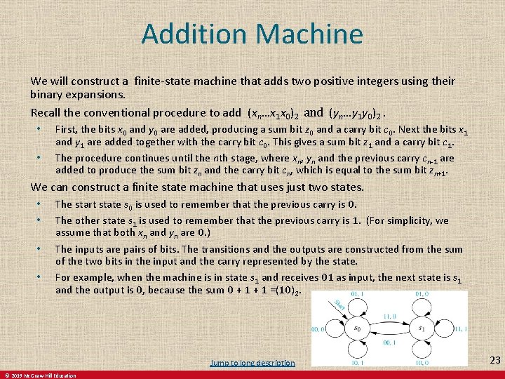
Addition Machine We will construct a finite-state machine that adds two positive integers using their binary expansions. Recall the conventional procedure to add (xn…x 1 x 0)2 and (yn…y 1 y 0)2. • • First, the bits x 0 and y 0 are added, producing a sum bit z 0 and a carry bit c 0. Next the bits x 1 and y 1 are added together with the carry bit c 0. This gives a sum bit z 1 and a carry bit c 1. The procedure continues until the nth stage, where xn, yn and the previous carry cn-1 are added to produce the sum bit zn and the carry bit cn, which is equal to the sum bit zn+1. We can construct a finite state machine that uses just two states. • • The start state s 0 is used to remember that the previous carry is 0. The other state s 1 is used to remember that the previous carry is 1. (For simplicity, we assume that both xn and yn are 0. ) The inputs are pairs of bits. The transitions and the outputs are constructed from the sum of the two bits in the input and the carry represented by the state. For example, when the machine is in state s 1 and receives 01 as input, the next state is s 1 and the output is 0, because the sum 0 + 1 =(10)2. Jump to long description © 2019 Mc. Graw-Hill Education 23

Finite-State Machines with No Output Section 13. 3 24 © 2019 Mc. Graw-Hill Education

Section Summary 3 Set of Strings Finite-State Automata Language Recognition by Finite-State Machines Designing Finite-State Automata Equivalent Finite-State Automata (not currently included in overheads) Nondeterministic Finite-State Automata 25 © 2019 Mc. Graw-Hill Education

Set of Strings Stephen Cole Kleene (1909 -1994) FSMs with no output, but with some states designated as accepting states, are specifically designed for recognizing languages. The concatenation of A and B, where A and B are subsets of V*, denoted by AB, is the set of all strings of the form xy, where x is a string in A and y is a string in B. Let A = {0, 11} and B = {1, 10, 110}. Then AB = {01, 010, 0110, 111, 110, 11110} and BA = {10, 111, 100, 1011, 1100, 11011} If A is a subset of V*, the Kleene closure of A, denoted by A*, is the set consisting of arbitrarily long strings of elements of A. That is, The Kleene closures of the sets A = {0}, B = {0, 1} and C = {11} are 26 © 2019 Mc. Graw-Hill Education

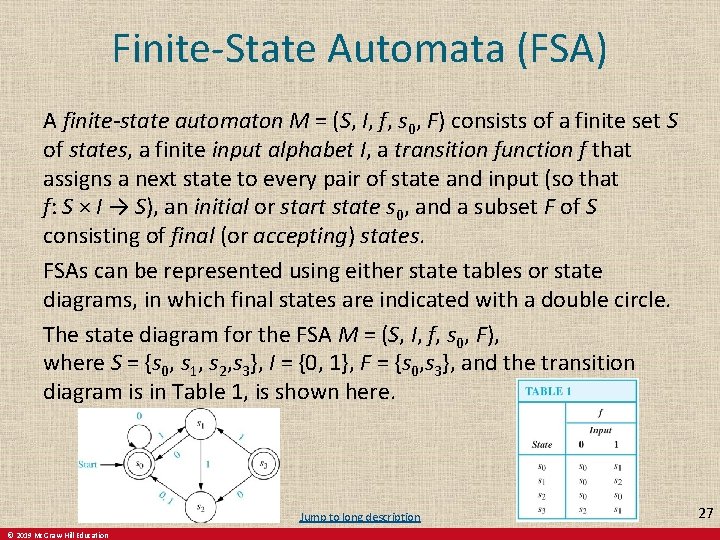
Finite-State Automata (FSA) A finite-state automaton M = (S, I, f, s 0, F) consists of a finite set S of states, a finite input alphabet I, a transition function f that assigns a next state to every pair of state and input (so that f: S × I → S), an initial or start state s 0, and a subset F of S consisting of final (or accepting) states. FSAs can be represented using either state tables or state diagrams, in which final states are indicated with a double circle. The state diagram for the FSA M = (S, I, f, s 0, F), where S = {s 0, s 1, s 2, s 3}, I = {0, 1}, F = {s 0, s 3}, and the transition diagram is in Table 1, is shown here. Jump to long description © 2019 Mc. Graw-Hill Education 27

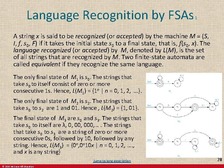
Language Recognition by FSAs 1 A string x is said to be recognized (or accepted) by the machine M = (S, I, f, s 0, F) if it takes the initial state s 0 to a final state, that is, f(s 0, x). The language recognized (or accepted) by M, denoted by L(M), is the set of all strings that are recognized by M. Two finite-state automata are called equivalent if they recognize the same language. The only final state of M 1 is s 0. The strings that take s 0 to itself consist of zero or more consecutive 1 s. Hence, L(M 1) = {1 n | n = 0, 1, 2, …. }. The only final state of M 2 is s 2. The strings that take s 0 to s 2 are 1 and 01. Hence , L(M 2) = {1, 01}. The final state of M 3 are s 0 and s 3. The strings that take s 0 to itself are λ, 0, 000, …. The strings that take s 0 to s 3 are a string of zero or more consecutive 0 s, followed by 10, followed by any string. Hence, L(M 3) = {0 n, 0 n 10 x | n = 0, 1, 2, …. , and x is any string} Jump to long description © 2019 Mc. Graw-Hill Education 28

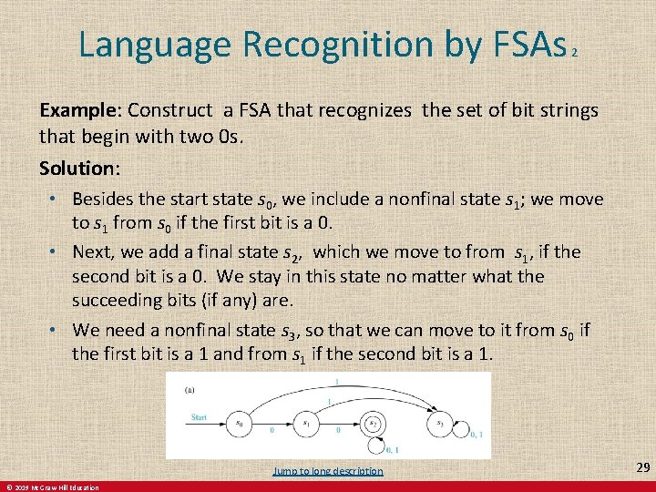
Language Recognition by FSAs 2 Example: Construct a FSA that recognizes the set of bit strings that begin with two 0 s. Solution: • Besides the start state s 0, we include a nonfinal state s 1; we move to s 1 from s 0 if the first bit is a 0. • Next, we add a final state s 2, which we move to from s 1, if the second bit is a 0. We stay in this state no matter what the succeeding bits (if any) are. • We need a nonfinal state s 3, so that we can move to it from s 0 if the first bit is a 1 and from s 1 if the second bit is a 1. Jump to long description © 2019 Mc. Graw-Hill Education 29

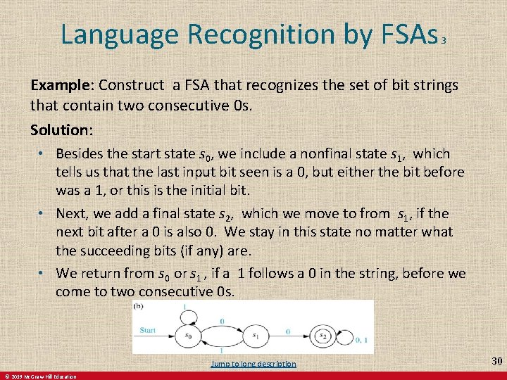
Language Recognition by FSAs 3 Example: Construct a FSA that recognizes the set of bit strings that contain two consecutive 0 s. Solution: • Besides the start state s 0, we include a nonfinal state s 1, which tells us that the last input bit seen is a 0, but either the bit before was a 1, or this is the initial bit. • Next, we add a final state s 2, which we move to from s 1, if the next bit after a 0 is also 0. We stay in this state no matter what the succeeding bits (if any) are. • We return from s 0 or s 1 , if a 1 follows a 0 in the string, before we come to two consecutive 0 s. Jump to long description © 2019 Mc. Graw-Hill Education 30

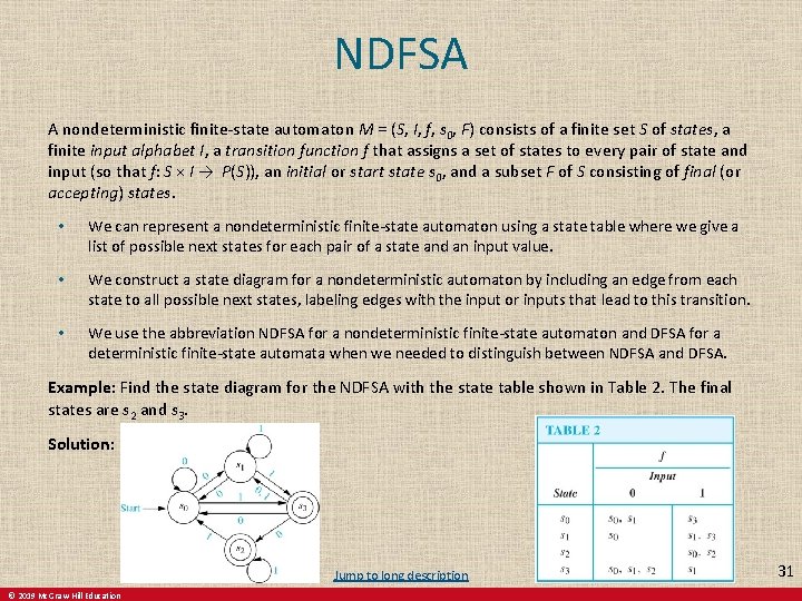
NDFSA A nondeterministic finite-state automaton M = (S, I, f, s 0, F) consists of a finite set S of states, a finite input alphabet I, a transition function f that assigns a set of states to every pair of state and input (so that f: S × I → P(S)), an initial or start state s 0, and a subset F of S consisting of final (or accepting) states. • We can represent a nondeterministic finite-state automaton using a state table where we give a list of possible next states for each pair of a state and an input value. • We construct a state diagram for a nondeterministic automaton by including an edge from each state to all possible next states, labeling edges with the input or inputs that lead to this transition. • We use the abbreviation NDFSA for a nondeterministic finite-state automaton and DFSA for a deterministic finite-state automata when we needed to distinguish between NDFSA and DFSA. Example: Find the state diagram for the NDFSA with the state table shown in Table 2. The final states are s 2 and s 3. Solution: Jump to long description © 2019 Mc. Graw-Hill Education 31

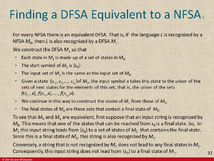
Finding a DFSA Equivalent to a NFSA 1 32 © 2019 Mc. Graw-Hill Education

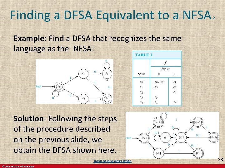
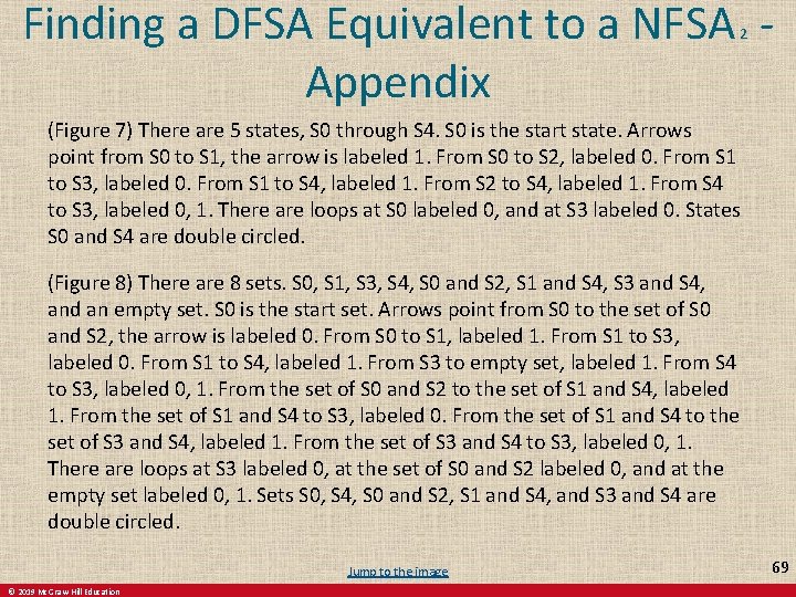
Finding a DFSA Equivalent to a NFSA 2 Example: Find a DFSA that recognizes the same language as the NFSA: Solution: Following the steps of the procedure described on the previous slide, we obtain the DFSA shown here. Jump to long description © 2019 Mc. Graw-Hill Education 33

Language Recognition Section 13. 4 34 © 2019 Mc. Graw-Hill Education

Section Summary 4 Regular Expressions Kleene’s Theorem Regular Sets and Regular Grammars More Powerful Types of Machines 35 © 2019 Mc. Graw-Hill Education

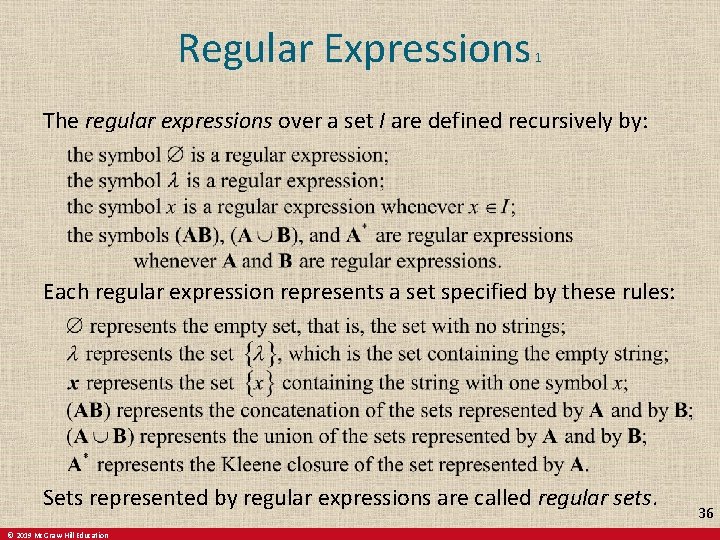
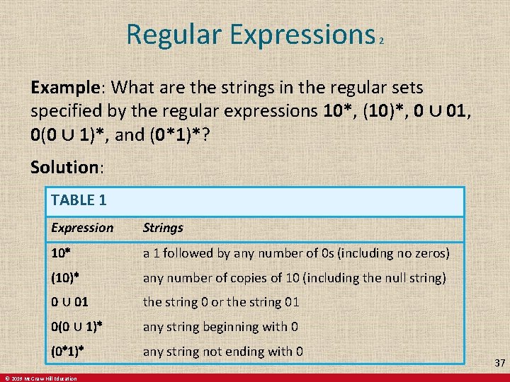
Regular Expressions 1 The regular expressions over a set I are defined recursively by: Each regular expression represents a set specified by these rules: Sets represented by regular expressions are called regular sets. © 2019 Mc. Graw-Hill Education 36

Regular Expressions 2 Example: What are the strings in the regular sets specified by the regular expressions 10*, (10)*, 0 ∪ 01, 0(0 ∪ 1)*, and (0*1)*? Solution: TABLE 1 Expression Strings 10∗ a 1 followed by any number of 0 s (including no zeros) (10)∗ any number of copies of 10 (including the null string) 0 ∪ 01 the string 0 or the string 01 0(0 ∪ 1)∗ any string beginning with 0 (0∗ 1)∗ any string not ending with 0 © 2019 Mc. Graw-Hill Education 37

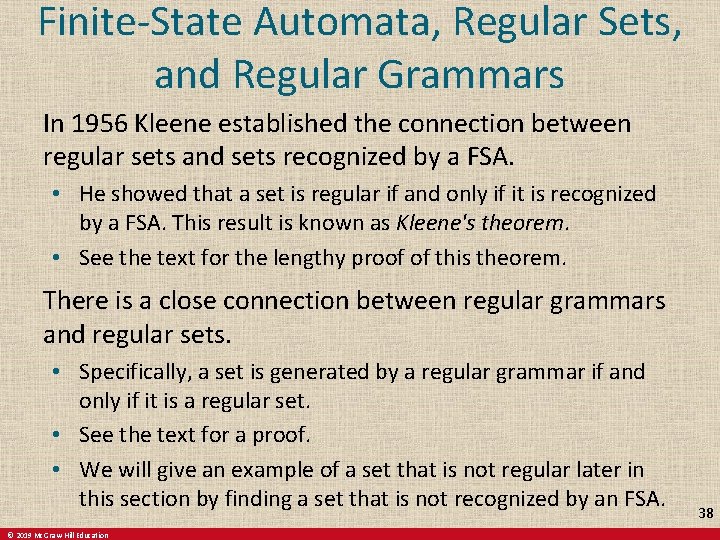
Finite-State Automata, Regular Sets, and Regular Grammars In 1956 Kleene established the connection between regular sets and sets recognized by a FSA. • He showed that a set is regular if and only if it is recognized by a FSA. This result is known as Kleene's theorem. • See the text for the lengthy proof of this theorem. There is a close connection between regular grammars and regular sets. • Specifically, a set is generated by a regular grammar if and only if it is a regular set. • See the text for a proof. • We will give an example of a set that is not regular later in this section by finding a set that is not recognized by an FSA. © 2019 Mc. Graw-Hill Education 38

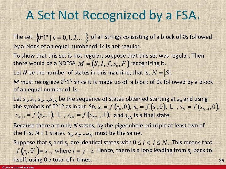
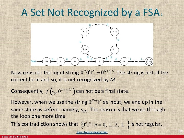
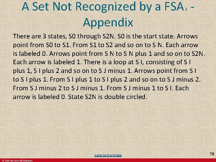
A Set Not Recognized by a FSA The set 1 of all strings consisting of a block of 0 s followed by a block of an equal number of 1 s is not regular. To show that this set is not regular, suppose that this set was regular. Then recognizing it. there would be a NDFSA Let N be the number of states in this machine, that is, M must recognize 0 N 1 N since it is made up of a block of 0 s followed by a block of an equal number of 1 s. Let s 0, s 1, s 2, …, s 2 N be the sequence of states obtained starting at s 0 and using the symbols of 0 N 1 N as input. So, and s 2 N is a final state. Because there are only N states, by the pigeonhole principle at least two of the first N + 1 states s 0, s 2, …, s. N must be the same. Suppose that si and sj are identical states with This means that Hence, there is a loop leading from si back to itself, using 0 a total of t times. © 2019 Mc. Graw-Hill Education 39

A Set Not Recognized by a FSA 2 Now consider the input string The string is not of the correct form and so, it is not recognized by M. Consequently, can not be a final state. However, when we use the string as input, we end up in the same state as before, namely, s 2 N. The reason is that we go through the loop one more time. This contradiction shows that is not regular. Jump to long description © 2019 Mc. Graw-Hill Education 40

More Powerful Types of Machines The main limitation of finite-state automata is their finite amount of memory. This has led to the development of more powerful types of machines. • Pushdown Automaton (PDA): includes a stack, which provides unlimited memory. We can use a PDA to recognize but no PDA recognizes the set • Linear Bounded Automaton (LBA): More powerful than pushdown automata. We can use a LBA to recognize but there are languages generated by phrase-structure grammars that cannot be recognized by a LBA. • Turing Machine (TM): Yet more powerful machines (to be studied in the next section) which can recognize all languages generated by phrase-structure grammars. © 2019 Mc. Graw-Hill Education 41

Turing Machines Section 13. 5 42 © 2019 Mc. Graw-Hill Education

Section Summary 5 Definition of Turing Machines Using Turing Machines to Recognize Sets Computing Functions with Turing Machines Different Types of Turing Machines (not currently included in overheads) The Church-Turing Thesis Computational Complexity, Computability, and Decidability © 2019 Mc. Graw-Hill Education

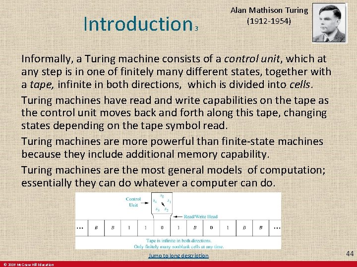
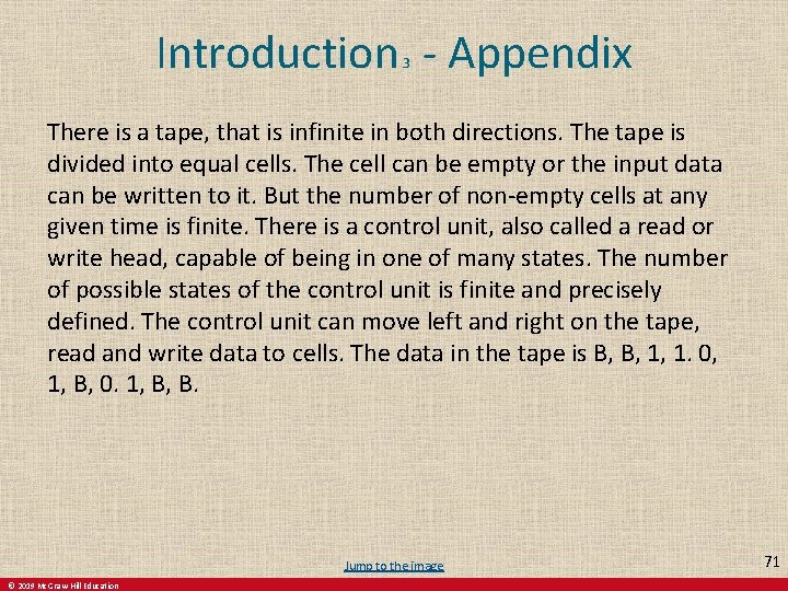
Introduction 3 Alan Mathison Turing (1912 -1954) Informally, a Turing machine consists of a control unit, which at any step is in one of finitely many different states, together with a tape, infinite in both directions, which is divided into cells. Turing machines have read and write capabilities on the tape as the control unit moves back and forth along this tape, changing states depending on the tape symbol read. Turing machines are more powerful than finite-state machines because they include additional memory capability. Turing machines are the most general models of computation; essentially they can do whatever a computer can do. Jump to long description © 2019 Mc. Graw-Hill Education 44

Definition of Turing Machines (TM) A Turing machine T = (S, I, f, s 0) consists of • a finite set S of states, • an alphabet I containing the blank symbol B, • a partial function f from S × I to S × I ×{R, L}, and • a starting state s 0. For some (state, symbol) pairs the partial function f may be undefined, but for a pair for which it is defined, there is a unique (state, symbol, direction) triple associated to this pair. The five-tuples corresponding to the partial function in the definition of a TM are called the transition rules of the machine. At each step, the control unit reads the current tape symbol x. If the control unit is in state s and if the partial function f is defined for the pair (s, x) with f(s, x) = (s′, x′, d), the control unit: • enters the state s′, • writes the symbol x′ in the current cell, erasing x, and • moves right one cell if d = R or moves left one cell if d = L. This step is written as the five-tuple (s, x, s′, x′, d). Turing machines are defined by specifying a set of such five-tuples. If the partial function f is undefined for the pair (s, x) then T will halt. At the beginning of its operation a TM is assumed to be in the initial state s 0 and to be positioned over the leftmost nonblank symbol on the tape. This is the initial position of the machine. © 2019 Mc. Graw-Hill Education 45

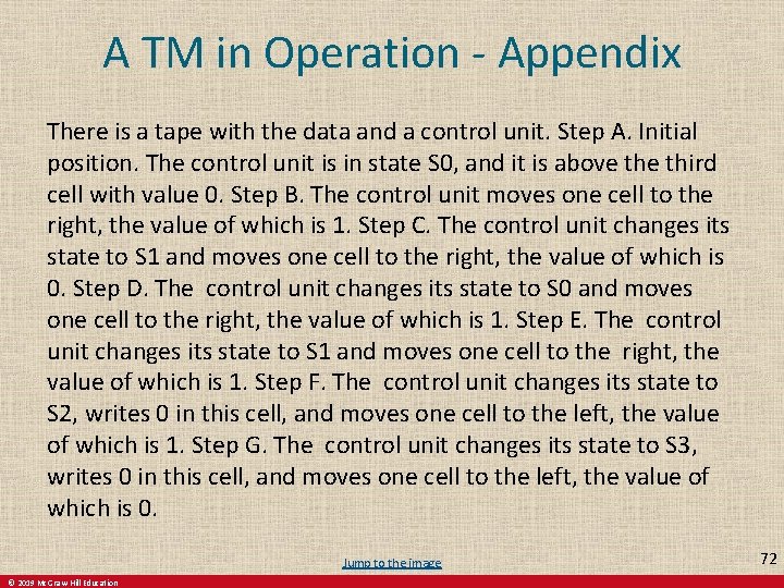
A TM in Operation Example: What is the final tape when the TM T defined by the seven five-tuples (s 0, 0, R), (s 0, 1, s 1, 1, R), (s 0, B, s 3, B, R), (s 1, 0, s 0, 0, R), (s 1, s 2, 0, L), (s 1, B, s 3, B, R), and (s 2, 1, s 3, 0, R) is run on the tape shown here in (a)? Solution: The transitions of this TM are shown to the right. The final tape is shown in (g). Jump to long description © 2019 Mc. Graw-Hill Education 46

Using TM to Recognize Sets 1 Let V be a subset of an alphabet I. A TM T = (S, I, f, s 0) recognizes a string x in V* if and only if T, starting in the initial position when x is written on the tape, halts in a final state. T is said to recognize a subset A of V* if x is recognized by T if and only if x belongs to A. Note that to recognize a subset A of V* we can use symbols not in V. This means that the input alphabet I may include symbols not in V. We will see that these extra symbols are used as markers. A TM operating on a tape containing the symbols of a string x in consecutive cells, does not recognize x if it does not halt or halts in a state that is not final. © 2019 Mc. Graw-Hill Education 47

Using TMs to Recognize Sets 2 In Section 13. 4 we showed that there is no DFA that recognizes the set We will now construct a TM that recognizes this set. the set • We use an auxiliary tape symbol M as a marker, and specify that V = {0, 1} and I = {0, 1, M}. • Our TM has one final state, s 6. The TM successively replaces a 0 at the leftmost position of the string with an M and a 1 at the rightmost position of the string with an M, sweeping back and forth, terminating in a final state if and only if the string consists of a block of 0 s followed by a block of the same number of 1 s. • The five-tuples are (s 0, 0, s 1, M, R), (s 1, 0, R), (s 1, 1, R), (s 1, M, s 2, M, L), (s 1, B, s 2, B, L), (s 2, 1, s 3, M, L), (s 3, 1, L), (s 3, 0, s 4, 0, L), (s 3, M, s 5, M, R), (s 4, 0, L), (s 4, M, s 0, M, R), and (s 5, M, s 6, M, R). For example, the string 000111 would successively become M 00111, M 0011 M, MM 01 MM, MMMMMM as the machine operates until it halts. © 2019 Mc. Graw-Hill Education 48

Computing Functions with TMs 1 A Turing machine can be used to compute the values of a partial function. Suppose that the TM T, when given the string x as input, halts with the string y on its tape. We can then define T(x) = y. To consider a TM as a computer of functions from the set of k-tuples of nonnegative integers to the set of nonnegative integers, we use the unary representation of integers. A nonnegative integer n is represented by a string of n + 1 1 s. So, 0 is represented by 1, 5 by 111111, etc. To represent an input that is a k-tuple of integers, we represent each integer in the k-tuple separately and separate these representations using asterisks. For example, (2, 0, 1, 3) is represented by 111*1*11*1111. Constructing a Turing machine that computes a particular function can be extremely complicated. Fortunately, the ability of Turing machines to compute functions is of theoretical, rather than practical, interest. 49 © 2019 Mc. Graw-Hill Education

Computing Functions with TMs 2 To construct a TM T that computes the function we first represent the pair (n 1, n 2) by a string of n 1 + 1 1 s followed by an asterisk, followed by n 2 + 1 1 s. The machine starts at the leftmost 1 of the input string, and proceeds to erase this 1. If the next character is an asterisk, n 1 = 0. In this case, it replaces the asterisk with a blank and halts. Otherwise, it erases the next 1, and then passes over the remaining 1 s, until it comes to the asterisk. The asterisk is then replaced by a 1. The five-tuples defining this Turing machine are: (s 0, 1, s 1, B, R), (s 1, ∗, s 3, B, R), (s 1, 1, s 2, B, R), (s 2, 1, R), (s 2, ∗, s 3, 1, R). © 2019 Mc. Graw-Hill Education 50

The Church-Turing Thesis says that given any problem that can be solved with an effective algorithm, there is a TM that can solve this problem. It is called a thesis rather than a theorem because the concept of solvability by an effective algorithm is informal and imprecise, as opposed to the concept of solvability by a TM, which is formal and precise. 51 © 2019 Mc. Graw-Hill Education

Decidability and Complexity A decision problem asks whether statements from a particular class of statements are true. Decision problems are also known as yes-or-no problems. • • Consider the question for a particular integer n, “Is n prime? ” The answer is "yes" or "no. “ The halting problem is the decision problem that asks whether a Turing machine T eventually halts when given an input string x. When there is an effective algorithm that decides whether instances of a decision problem are true, we say that this problem is solvable or decidable. • In Section 3. 5, an algorithm was given for determining whether a positive integer n is prime by checking whether it is divisible by primes not exceeding its square root. However, if no effective algorithm exists for solving a problem, then we say the problem is unsolvable or undecidable. • The halting problem is an unsolvable decision problem (proved in Section 3. 1). That is, no TM exists that, when given an encoding of a TM T and its input string x as input, can determine whether T eventually halts when started with x written on its tape. A function that can be computed by a TM is called computable and a function that cannot be computed by a TM is called uncomputable. • The busy beaver function, which when given a positive integer n gives the maximum number of 1 s that a TM with n states and alphabet {1, B} may print on an initially blank tape is uncomputable (see Exercise 35 in Section 13. 5). 52 © 2019 Mc. Graw-Hill Education

The Classes P and NP 1 In a nondeterministic Turing machine (NDTM), the restriction that no two transition rules begin with the same pair (s, x) is eliminated. Hence, there may be more than one transition rule beginning with each (state, tape symbol) pair, so that there may be a choice as to which rule to use at each step. A NDTM T recognizes a string x if and only if there exists some sequence of transitions of T that ends in a final state when the machine starts in the initial position with x written on the tape. © 2019 Mc. Graw-Hill Education 53

The Classes P and NP 2 A decision problem is in P, the class of polynomial-time problems, if it can be solved by a deterministic Turing machine in polynomial time in terms of the size of its input. That is, a decision problem is in P if there is a deterministic Turing machine T that solves the decision problem and a polynomial p(n) such that for all integers n, T halts in a final state after no more than p(n) transitions whenever the input to T is a string of length n. A decision problem is in NP, the class of nondeterministic polynomial-time problems, if it can be solved by a nondeterministic Turing machine in polynomial time in terms of the size of its input. That is, a decision problem is in NP if there is a nondeterministic Turing machine T that solves the problem and a polynomial p(n) such that for all integers n, T halts for every choice of transitions after no more than p(n) transitions whenever the input to T is a string of length n. Problems in P are called tractable, whereas problems not in P are called intractable. 54 © 2019 Mc. Graw-Hill Education

The Classes P and NP 3 For a problem to be in NP, it is necessary only that there be a NDTM that when given a true statement from the set of statements addressed by the problem, can verify its truth in polynomial time by making the correct guess at each step. • The problem of determining whether a given graph has a Hamilton circuit is an NP problem, because a NDTM can easily verify that a simple circuit in a graph passes through each vertex exactly once. • It can do this by making a series of correct guesses corresponding to successively adding edges to form the circuit. 55 © 2019 Mc. Graw-Hill Education

Wrapping Everything up with a Millennium Problem Because every DTM can also be a considered to be a NDTM, where each (state, tape symbol) pair occurs in exactly one transition rule, The most famous open question in theoretical CS, and one of the millennium problems with a $1, 000 prize, is whether every problem in NP is also in P, that is, whether P = NP. There is an important class of problems, known as NP-complete problems, where a problem is in this class if it is the class NP and if this problem was also in the class P, then every problem in NP must also be in P. That is, a problem is NP-complete if the existence of a polynomial-time algorithm for solving it implies the existence of a polynomial-time algorithm for every problem in NP. We have studied several problems that can be shown to be NP-complete in this text, including determining whether a simple graph has a Hamilton circuit and determining whether a proposition in n variables is a tautology. This concludes our introduction to discrete mathematics, but it should come as no surprise that there is a lot more to learn! © 2019 Mc. Graw-Hill Education 56

57 © 2019 Mc. Graw-Hill Education

Appendix of Image Long Descriptions 58 © 2019 Mc. Graw-Hill Education

Derivation Trees- Appendix The root of this tree is sentence. The nodes of the root are noun phrase and verb phrase. Noun phrase is divided into article, adjective, and noun. Article is the, adjective is hungry, noun is rabbit. Verb phrase is divided into verb and adverb. Verb is eats. Adverb is quickly. Jump to the image © 2019 Mc. Graw-Hill Education 59

An Example of a Finite-State Machine with Output - Appendix 2 There are 7 states, S 0 through S 6. S 0 is the start state. The states are presented as circles. Arrows point from S 0 to S 1, the arrow is labeled 5, N. From S 0 to S 2, labeled 10, N. From S 0 to S 5, labeled 25, N. From S 1 to S 2, labeled 5, N. From S 1 to S 3, labeled 10, N. From S 1 to S 6, labeled 25, N. From S 2 to S 3, labeled 5, N. From S 2 to S 4, labeled 10, N. From S 2 to S 6, labeled 25, 5. From S 3 to S 4, labeled 5, N. From S 3 to S 5, labeled 10, N. From S 3 to S 6, labeled 25, 10. From S 4 to S 5, labeled 5, N. From S 4 to S 6, labeled 10, N. From S 4 to S 6, labeled 25, 15. There are 3 arrows from S 5 to S 6, labeled 5, N, 10, 5, and 25, 20. There are 2 arrows from S 6 to S 0, labeled O, orange juice and R, apple juice. The states, S 0 through S 5 have a loops, each labeled R, N, O, N. State S 6 has 3 loops, labeled 5, 5, 10, and 25, 25. Jump to the image © 2019 Mc. Graw-Hill Education 60

FSMs with Outputs - Appendix There are 4 states, S 0 through S 3. S 0 is the start state. Arrows point from S 0 to S 1, the arrow is labeled 0, 1. From S 1 to S 0, labeled 1, 1. From S 1 to S 3, labeled 0, 1. From S 2 to S 1, labeled 0, 0. From S 3 to S 1, labeled 1, 0. From S 3 to S 2, labeled 0, 0. There are loops at S 0 labeled 1, 0, and at S 2 labeled 1, 1. Jump to the image © 2019 Mc. Graw-Hill Education 61

Unit-delay Machine - Appendix There are 3 states, S 0 through S 2. S 0 is the start state. Arrows point from S 0 to S 1, the arrow is labeled 1, 0. From S 0 to S 2, labeled 0, 0. From S 1 to S 2, labeled 0, 1. From S 2 to S 1, labeled 1, 0. There are loops at S 1 labeled 1, 1, and at S 2 labeled 0, 0. Jump to the image © 2019 Mc. Graw-Hill Education 62

Addition Machine - Appendix There are 2 states, S 0 and S 1. S 0 is the start state. Arrows point from S 0 to S 1, the arrow is labeled 11, 0. From S 1 to S 0, labeled 00, 1. There are 3 loops at S 0, labeled 00, 0. 01, 1, and 10, 1. There are 3 loops at S 1, labeled 01, 0. 10, 0, and 11, 1. Jump to the image © 2019 Mc. Graw-Hill Education 63

Finite-State Automata (FSA) - Appendix There are 4 states, S 0 through S 3. S 0 is the start state. Arrows point from S 0 to S 1, the arrow is labeled 1. From S 1 to S 0, labeled 0. From S 1 to S 2, labeled 1. From S 2 to S 0, labeled 0, 1. From S 3 to S 1, labeled 1. From S 3 to S 2, labeled 0. There is a loop at S 0, labeled 0. States S 0 and S 3 are double circled. Jump to the image © 2019 Mc. Graw-Hill Education 64

Language Recognition by FSAs - Appendix 1 Diagram M 1. There are 2 states, S 0 and S 1. S 0 is the start state. Arrows points from S 0 to S 1, the arrow is labeled 0. There is a loop at S 0, labeled 1. State S 0 is double circled. Diagram M 2. There are 4 states, S 0 through S 3. S 0 is the start state. Arrows point from S 0 to S 1, the arrow is labeled 0. From S 0 to S 2, labeled 1. From S 1 to S 2, labeled 1. From S 1 to S 3, labeled 0. From S 2 to S 3, labeled 0, 1. There is a loop at S 3, labeled 0, 1. State S 2 is double circled. Diagram M 3. There are 4 states, S 0 through S 3. S 0 is the start state. Arrows point from S 0 to S 1, the arrow is labeled 1. From S 1 to S 2, labeled 1. From S 1 to S 3, labeled 0. There are loops at S 0 labeled 0, at S 2 labeled 0, 1, and at S 3 labeled 0, 1. States S 0 and S 3 are double circled. Jump to the image © 2019 Mc. Graw-Hill Education 65

Language Recognition by FSAs - Appendix 2 There are 4 states, S 0 through S 3. S 0 is the start state. Arrows point from S 0 to S 1, the arrow is labeled 0. From S 0 to S 3, labeled 1. From S 1 to S 2, labeled 0. From S 1 to S 3, labeled 1. There are loops at S 2 labeled 0, 1, and at S 3 labeled 0, 1. State S 2 is double circled. Jump to the image © 2019 Mc. Graw-Hill Education 66

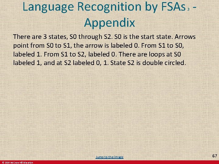
Language Recognition by FSAs - Appendix 3 There are 3 states, S 0 through S 2. S 0 is the start state. Arrows point from S 0 to S 1, the arrow is labeled 0. From S 1 to S 0, labeled 1. From S 1 to S 2, labeled 0. There are loops at S 0 labeled 1, and at S 2 labeled 0, 1. State S 2 is double circled. Jump to the image © 2019 Mc. Graw-Hill Education 67

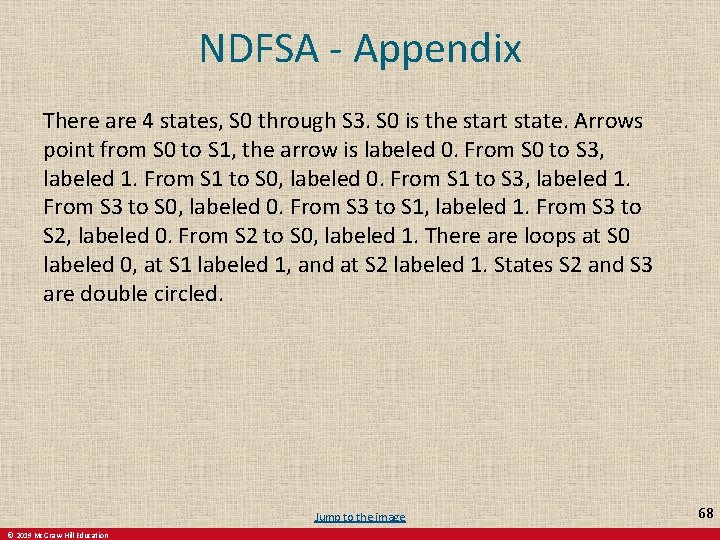
NDFSA - Appendix There are 4 states, S 0 through S 3. S 0 is the start state. Arrows point from S 0 to S 1, the arrow is labeled 0. From S 0 to S 3, labeled 1. From S 1 to S 0, labeled 0. From S 1 to S 3, labeled 1. From S 3 to S 0, labeled 0. From S 3 to S 1, labeled 1. From S 3 to S 2, labeled 0. From S 2 to S 0, labeled 1. There are loops at S 0 labeled 0, at S 1 labeled 1, and at S 2 labeled 1. States S 2 and S 3 are double circled. Jump to the image © 2019 Mc. Graw-Hill Education 68

Finding a DFSA Equivalent to a NFSA - Appendix 2 (Figure 7) There are 5 states, S 0 through S 4. S 0 is the start state. Arrows point from S 0 to S 1, the arrow is labeled 1. From S 0 to S 2, labeled 0. From S 1 to S 3, labeled 0. From S 1 to S 4, labeled 1. From S 2 to S 4, labeled 1. From S 4 to S 3, labeled 0, 1. There are loops at S 0 labeled 0, and at S 3 labeled 0. States S 0 and S 4 are double circled. (Figure 8) There are 8 sets. S 0, S 1, S 3, S 4, S 0 and S 2, S 1 and S 4, S 3 and S 4, and an empty set. S 0 is the start set. Arrows point from S 0 to the set of S 0 and S 2, the arrow is labeled 0. From S 0 to S 1, labeled 1. From S 1 to S 3, labeled 0. From S 1 to S 4, labeled 1. From S 3 to empty set, labeled 1. From S 4 to S 3, labeled 0, 1. From the set of S 0 and S 2 to the set of S 1 and S 4, labeled 1. From the set of S 1 and S 4 to S 3, labeled 0. From the set of S 1 and S 4 to the set of S 3 and S 4, labeled 1. From the set of S 3 and S 4 to S 3, labeled 0, 1. There are loops at S 3 labeled 0, at the set of S 0 and S 2 labeled 0, and at the empty set labeled 0, 1. Sets S 0, S 4, S 0 and S 2, S 1 and S 4, and S 3 and S 4 are double circled. Jump to the image © 2019 Mc. Graw-Hill Education 69

A Set Not Recognized by a FSA - Appendix 2 There are 3 states, S 0 through S 2 N. S 0 is the start state. Arrows point from S 0 to S 1. From S 1 to S 2 and so on to S N. Each arrow is labeled 0. Arrows point from S N to S N plus 1 and so on to S 2 N. Each arrow is labeled 1. There is a loop at S I, consisting of S I plus 1, S I plus 2 and so on to S J minus 1. Arrows point from S I to S I plus 1. From S I plus 1 to S I plus 2 and so on to S J minus 2. From S J minus 2 to S J minus 1. From S J minus 1 to S I. Each arrow is labeled 0. State S 2 N is double circled. Jump to the image © 2019 Mc. Graw-Hill Education 70

Introduction - Appendix 3 There is a tape, that is infinite in both directions. The tape is divided into equal cells. The cell can be empty or the input data can be written to it. But the number of non-empty cells at any given time is finite. There is a control unit, also called a read or write head, capable of being in one of many states. The number of possible states of the control unit is finite and precisely defined. The control unit can move left and right on the tape, read and write data to cells. The data in the tape is B, B, 1, 1. 0, 1, B, 0. 1, B, B. Jump to the image © 2019 Mc. Graw-Hill Education 71

A TM in Operation - Appendix There is a tape with the data and a control unit. Step A. Initial position. The control unit is in state S 0, and it is above third cell with value 0. Step B. The control unit moves one cell to the right, the value of which is 1. Step C. The control unit changes its state to S 1 and moves one cell to the right, the value of which is 0. Step D. The control unit changes its state to S 0 and moves one cell to the right, the value of which is 1. Step E. The control unit changes its state to S 1 and moves one cell to the right, the value of which is 1. Step F. The control unit changes its state to S 2, writes 0 in this cell, and moves one cell to the left, the value of which is 1. Step G. The control unit changes its state to S 3, writes 0 in this cell, and moves one cell to the left, the value of which is 0. Jump to the image © 2019 Mc. Graw-Hill Education 72