Structure Computation Structure Computation How to compute the

Structure Computation

Structure Computation • How to compute the position of a point in 3 space given its image in two views and the camera matrices of those two views • Use image correspondence to compute F; then find a pair of consistent camera matrices. • Assume these matrices are known exactly or with great accuracy as compared to the matching points in the two images.

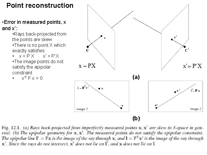
Point reconstruction • Error in measured points, x and x’: • Rays back-projected from the points are skew • There is no point X which exactly satisfies: • x=PX x’ = P’X • The image points do not satisfy the epipolar constraint • x’T F x = 0 (a) (b)

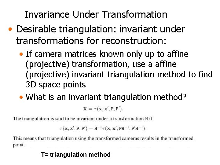
Invariance Under Transformation • Desirable triangulation: invariant under transformations for reconstruction: • If camera matrices known only up to affine (projective) transformation, use a affine (projective) invariant triangulation method to find 3 D space points • What is an invariant triangulation method? Τ= triangulation method

Projective Reconstruction • Inappropriate to minimize error in the 3 D projective space P 3 • Bad idea: find midpoint of the common perpendicular to the two rays in space: • Distance and perpendicularity not valid in projective geometry • Gives different results depending on which projective reconstruction is considered • Not projective invariant • Need to design a projective invariant approach • Better idea: minimize the re-projection error • Find 3 D point X so that the sum squared distance between the projection of X and measured image points x, and x’ is minimized

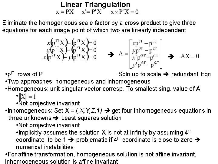
Linear Triangulation Eliminate the homogeneous scale factor by a cross product to give three equations for each image point of which two are linearly independent • pi. T rows of P Soln up to scale redundant Eqn • Two approaches: homogeneous and inhomogeneous • Homogeneous: unit singular vector corresp. To smallest sing. value of A • • Not projective invariant • Inhomogeneous: Set X = ( X, Y, Z, 1) get four inhomogeneous equations in three unknowns Least squares solution • Not projective invariant • Implicitly assumes the solution X is not at infinity by assuming 4 th coordinate to be 1 problematic if 4 th coordinate is close to zero numerical instabilities • For affine transformation, homogeneous solution is not affine invariant, inhomogeneous solution is affine invariant

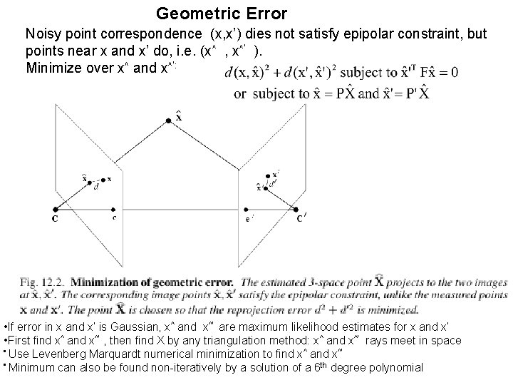
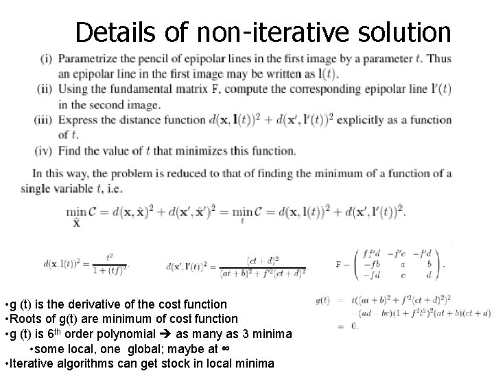
Geometric Error Noisy point correspondence (x, x’) dies not satisfy epipolar constraint, but points near x and x’ do, i. e. (x^ , x^’ ). Minimize over x^ and x^’: • If error in x and x’ is Gaussian, x^ and x^’ are maximum likelihood estimates for x and x’ • First find x^ and x^’ , then find X by any triangulation method: x^ and x^’ rays meet in space • Use Levenberg Marquardt numerical minimization to find x^ and x^’ • Minimum can also be found non-iteratively by a solution of a 6 th degree polynomial

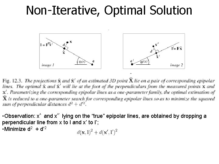
Non-Iterative, Optimal Solution • Observation: x^ and x^’ lying on the “true” epipolar lines, are obtained by dropping a perpendicular line from x to l and x’ to l’; • Minimize d 2 + d’ 2

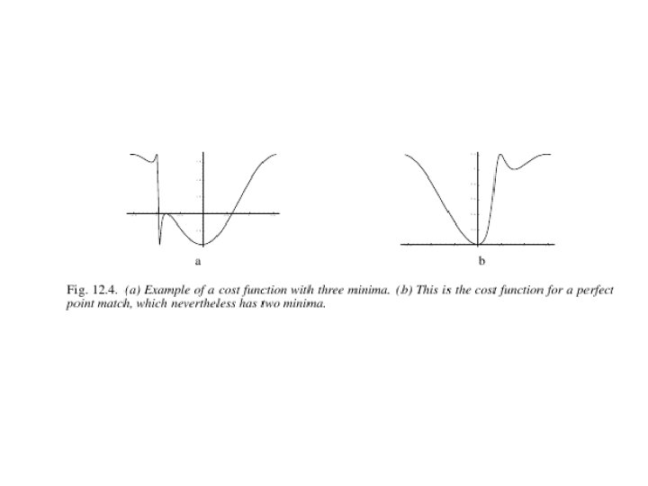
Details of non-iterative solution • g (t) is the derivative of the cost function • Roots of g(t) are minimum of cost function • g (t) is 6 th order polynomial as many as 3 minima • some local, one global; maybe at ∞ • Iterative algorithms can get stock in local minima

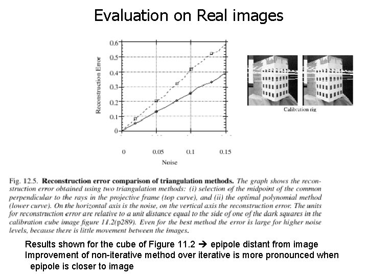
Evaluation on Real images Results shown for the cube of Figure 11. 2 epipole distant from image Improvement of non-iterative method over iterative is more pronounced when epipole is closer to image

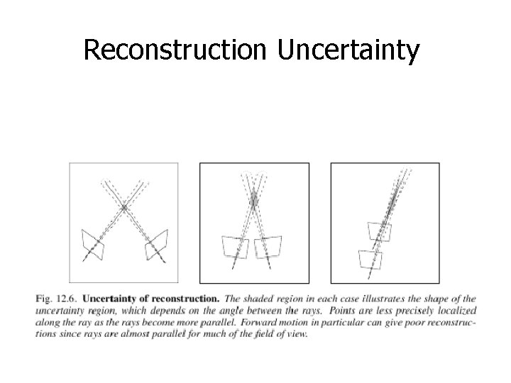
Reconstruction Uncertainty

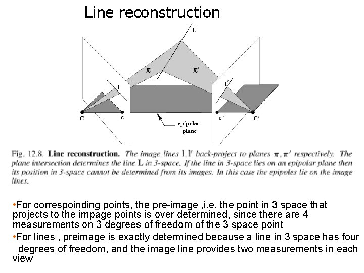
Line reconstruction • For correspoinding points, the pre-image , i. e. the point in 3 space that projects to the impage points is over determined, since there are 4 measurements on 3 degrees of freedom of the 3 space point • For lines , preimage is exactly determined because a line in 3 space has four degrees of freedom, and the image line provides two measurements in each view

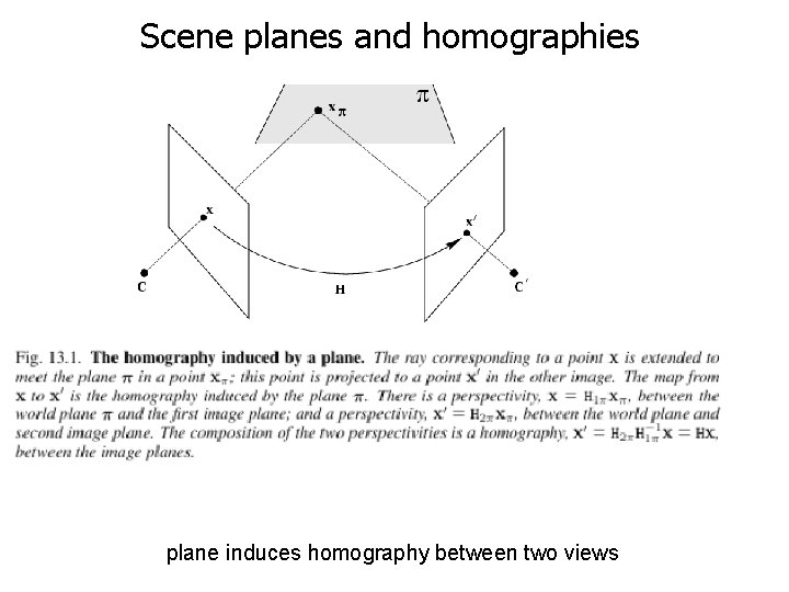
Scene planes and homographies plane induces homography between two views

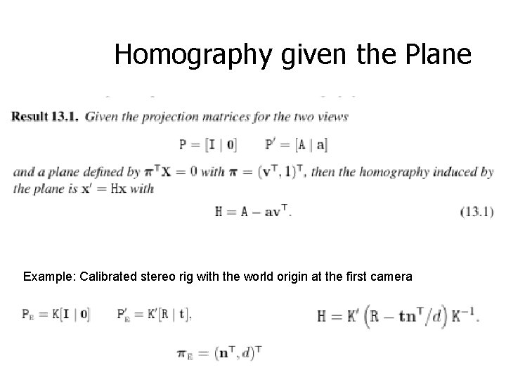
Homography given the Plane Example: Calibrated stereo rig with the world origin at the first camera

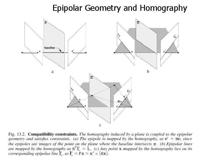
Epipolar Geometry and Homography

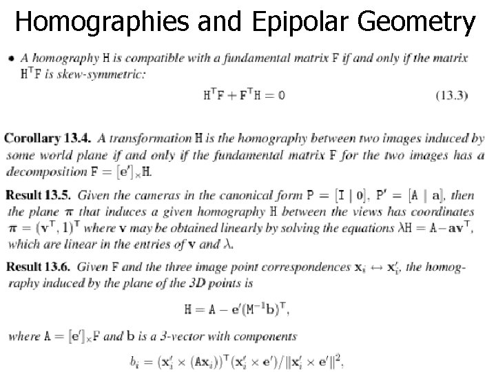
Homographies and Epipolar Geometry

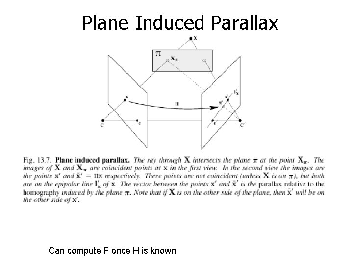
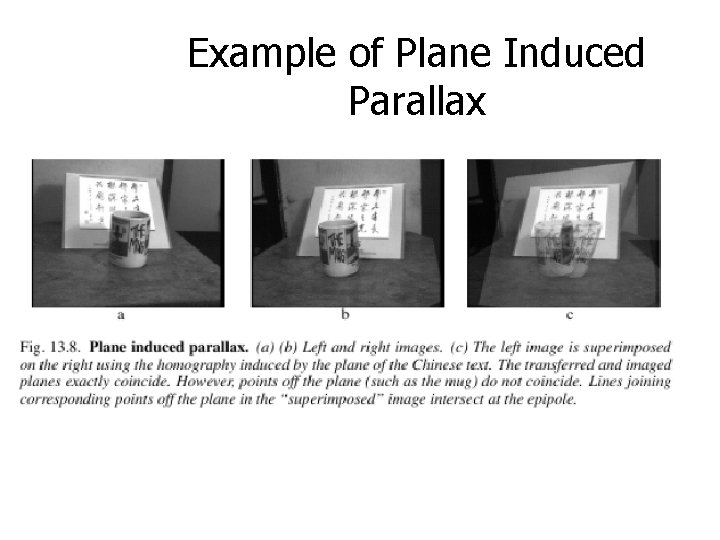
Plane Induced Parallax Can compute F once H is known

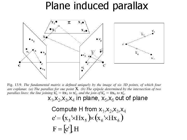
Plane induced parallax x 1, x 2, x 3, x 4 in plane, x 5, x 6 out of plane Compute H from x 1, x 2, x 3, x 4

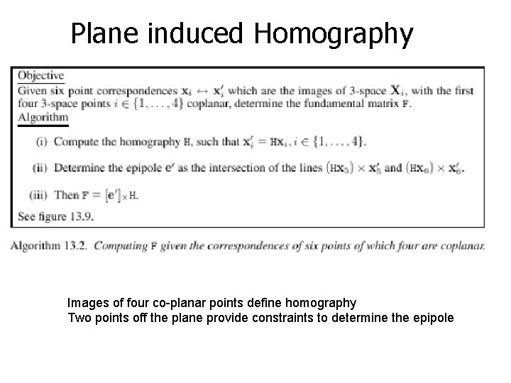
Plane induced Homography Images of four co-planar points define homography Two points off the plane provide constraints to determine the epipole

Example of Plane Induced Parallax