Chapter 4 Seasonal Series Forecasting and Decomposition Chapter

Chapter 4 Seasonal Series: Forecasting and Decomposition

Chapter 4: Seasonal Series: Forecasting and Decomposition 4. 1 Components of a Time Series 4. 2 Forecasting Purely Seasonal Series 4. 3 Forecasting Using a Seasonal Decomposition 4. 4 Pure Decomposition 4. 5 The Census X-13 Decomposition 4. 6 The Holt-Winters Seasonal Smoothing Methods 4. 7 The Multiplicative Holt-Winters Method 4. 8 Calculations Using R 4. 9 Weekly Data 4. 10 Prediction Intervals 4. 11 Principles for Seasonal Methods © 2017 Wessex Press, Inc. Principles of Business Forecasting 2 e (Ord, Fildes, Kourentzes) • Chapter 4: Seasonal Series: Forecasting and Decomposition 2

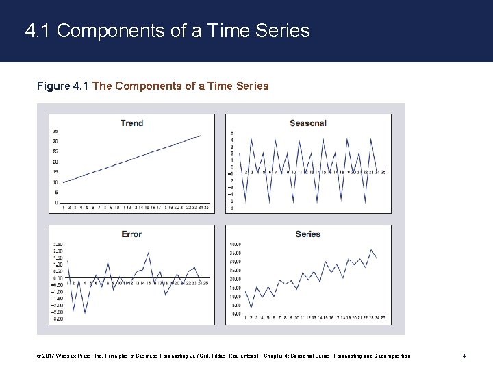
4. 1 Components of a Time Series • A time series is said to have a seasonal component if it displays a recurrent pattern with a fixed and known duration (e. g. months of the year, days of the week). • A time series is said to have a cyclical component if it displays somewhat regular fluctuations about the trend but those fluctuations have a random periodicity albeit with a constant mean period length (e. g. a business cycle). Define T = Trend + Cycle, S = Seasonal, E = Error • Additive model: Y = T + S + E • Multiplicative model: Y = TSE • Mixed additive-multiplicative model: Y = TS + E © 2017 Wessex Press, Inc. Principles of Business Forecasting 2 e (Ord, Fildes, Kourentzes) • Chapter 4: Seasonal Series: Forecasting and Decomposition 3

4. 1 Components of a Time Series Figure 4. 1 The Components of a Time Series © 2017 Wessex Press, Inc. Principles of Business Forecasting 2 e (Ord, Fildes, Kourentzes) • Chapter 4: Seasonal Series: Forecasting and Decomposition 4

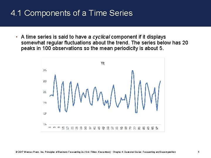
4. 1 Components of a Time Series • A time series is said to have a cyclical component if it displays somewhat regular fluctuations about the trend. The series below has 20 peaks in 100 observations so the mean periodicity is about 5. © 2017 Wessex Press, Inc. Principles of Business Forecasting 2 e (Ord, Fildes, Kourentzes) • Chapter 4: Seasonal Series: Forecasting and Decomposition 5

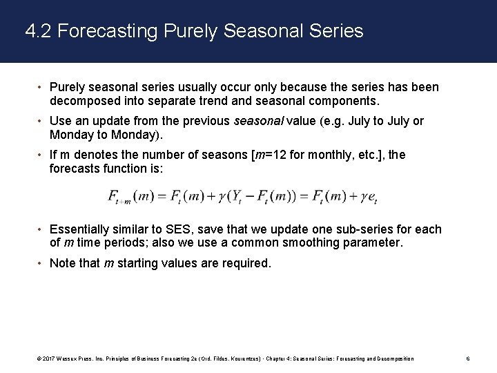
4. 2 Forecasting Purely Seasonal Series • Purely seasonal series usually occur only because the series has been decomposed into separate trend and seasonal components. • Use an update from the previous seasonal value (e. g. July to July or Monday to Monday). • If m denotes the number of seasons [m=12 for monthly, etc. ], the forecasts function is: • Essentially similar to SES, save that we update one sub-series for each of m time periods; also we use a common smoothing parameter. • Note that m starting values are required. © 2017 Wessex Press, Inc. Principles of Business Forecasting 2 e (Ord, Fildes, Kourentzes) • Chapter 4: Seasonal Series: Forecasting and Decomposition 6

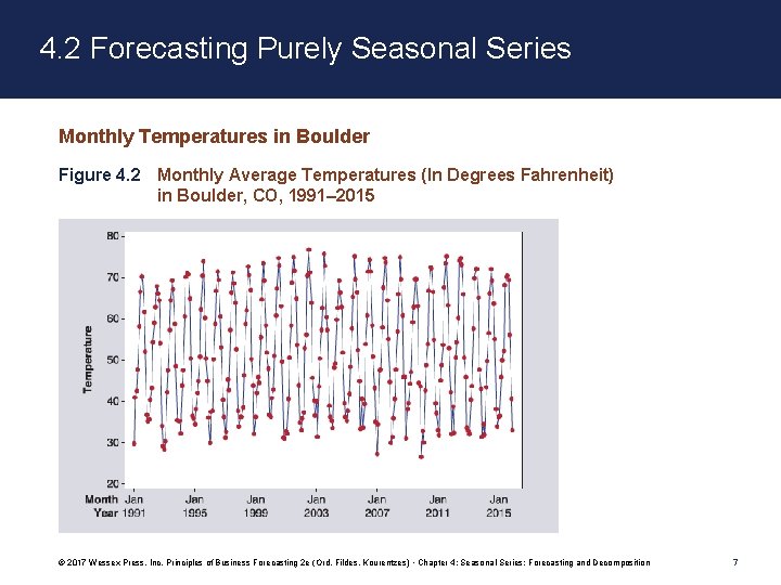
4. 2 Forecasting Purely Seasonal Series Monthly Temperatures in Boulder Figure 4. 2 Monthly Average Temperatures (In Degrees Fahrenheit) in Boulder, CO, 1991– 2015 © 2017 Wessex Press, Inc. Principles of Business Forecasting 2 e (Ord, Fildes, Kourentzes) • Chapter 4: Seasonal Series: Forecasting and Decomposition 7

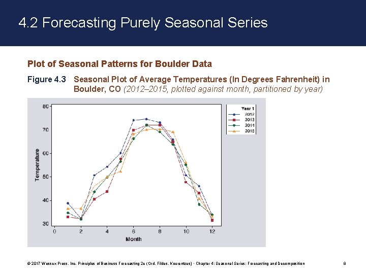
4. 2 Forecasting Purely Seasonal Series Plot of Seasonal Patterns for Boulder Data Figure 4. 3 Seasonal Plot of Average Temperatures (In Degrees Fahrenheit) in Boulder, CO (2012– 2015, plotted against month, partitioned by year) © 2017 Wessex Press, Inc. Principles of Business Forecasting 2 e (Ord, Fildes, Kourentzes) • Chapter 4: Seasonal Series: Forecasting and Decomposition 8

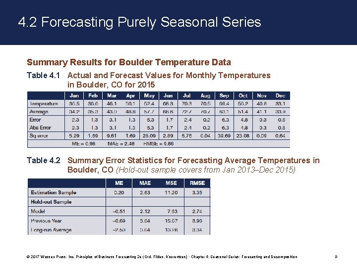
4. 2 Forecasting Purely Seasonal Series Summary Results for Boulder Temperature Data Table 4. 1 Actual and Forecast Values for Monthly Temperatures in Boulder, CO for 2015 Table 4. 2 Summary Error Statistics for Forecasting Average Temperatures in Boulder, CO (Hold-out sample covers from Jan 2013–Dec 2015) © 2017 Wessex Press, Inc. Principles of Business Forecasting 2 e (Ord, Fildes, Kourentzes) • Chapter 4: Seasonal Series: Forecasting and Decomposition 9

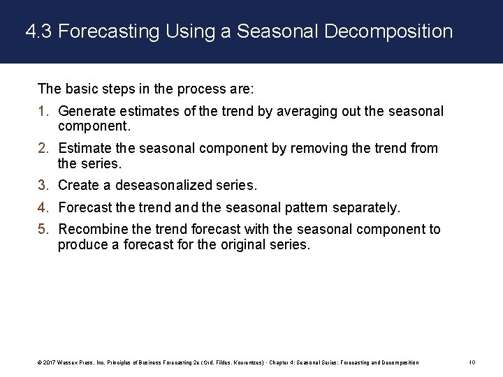
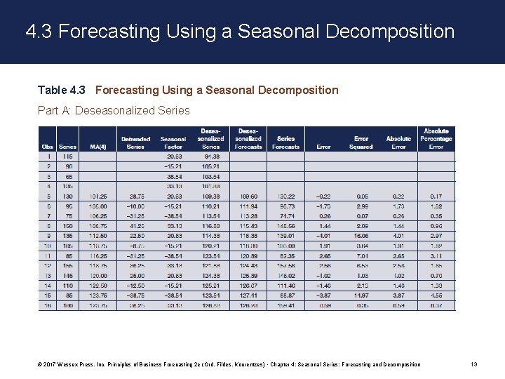
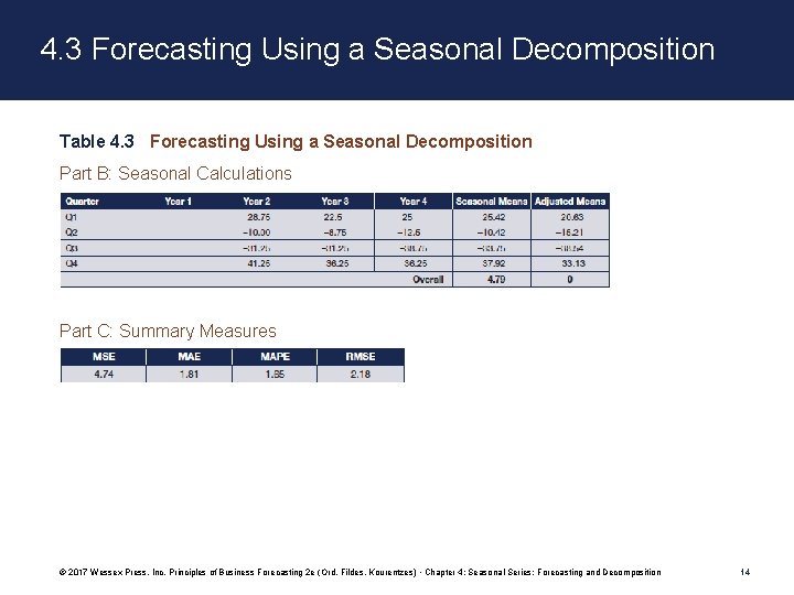
4. 3 Forecasting Using a Seasonal Decomposition The basic steps in the process are: 1. Generate estimates of the trend by averaging out the seasonal component. 2. Estimate the seasonal component by removing the trend from the series. 3. Create a deseasonalized series. 4. Forecast the trend and the seasonal pattern separately. 5. Recombine the trend forecast with the seasonal component to produce a forecast for the original series. © 2017 Wessex Press, Inc. Principles of Business Forecasting 2 e (Ord, Fildes, Kourentzes) • Chapter 4: Seasonal Series: Forecasting and Decomposition 10

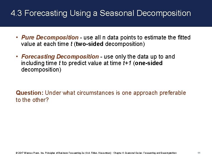
4. 3 Forecasting Using a Seasonal Decomposition • Pure Decomposition - use all n data points to estimate the fitted value at each time t (two-sided decomposition) • Forecasting Decomposition - use only the data up to and including time t to predict value at time t+1 (one-sided decomposition) Question: Under what circumstances is one approach preferable to the other? © 2017 Wessex Press, Inc. Principles of Business Forecasting 2 e (Ord, Fildes, Kourentzes) • Chapter 4: Seasonal Series: Forecasting and Decomposition 11

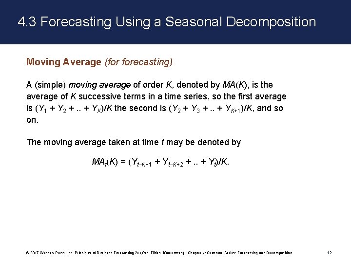
4. 3 Forecasting Using a Seasonal Decomposition Moving Average (for forecasting) A (simple) moving average of order K, denoted by MA(K), is the average of K successive terms in a time series, so the first average is (Y 1 + Y 2 +. . + YK)/K the second is (Y 2 + Y 3 +. . + YK+1)/K, and so on. The moving average taken at time t may be denoted by MAt(K) = (Yt–K+1 + Yt–K+2 +. . + Yt)/K. © 2017 Wessex Press, Inc. Principles of Business Forecasting 2 e (Ord, Fildes, Kourentzes) • Chapter 4: Seasonal Series: Forecasting and Decomposition 12

4. 3 Forecasting Using a Seasonal Decomposition Table 4. 3 Forecasting Using a Seasonal Decomposition Part A: Deseasonalized Series © 2017 Wessex Press, Inc. Principles of Business Forecasting 2 e (Ord, Fildes, Kourentzes) • Chapter 4: Seasonal Series: Forecasting and Decomposition 13

4. 3 Forecasting Using a Seasonal Decomposition Table 4. 3 Forecasting Using a Seasonal Decomposition Part B: Seasonal Calculations Part C: Summary Measures © 2017 Wessex Press, Inc. Principles of Business Forecasting 2 e (Ord, Fildes, Kourentzes) • Chapter 4: Seasonal Series: Forecasting and Decomposition 14

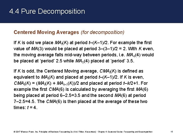
4. 4 Pure Decomposition Centered Moving Averages (for decomposition) If K is odd we place MAt(K) at period t–(K– 1)/2. For example the first value of MA(3) would be placed at period 3–(3– 1)/2 = 2. With K even, the moving average falls mid-way between periods, i. e. MA 4(4) would be placed at ‘period’ 2. 5 while MA 5(4) placed at ’period’ 3. 5. If K is odd, the Centered Moving average, CMAt(K) is defined as equivalent to MAt(K) and placed at period t–(K– 1)/2. If K is even, CMAt(K) = (MAt(K) + MAt+1(K))/2 and placed at period t–k/2+1. For example the first CMA(6) is calculated by averaging the first MA(6) being placed at period 6– 2. 5=3. 5 and the second MA(6) at period 7– 2. 5=4. 5. The CMA(6) is then placed at the average of these two times: t = 4. © 2017 Wessex Press, Inc. Principles of Business Forecasting 2 e (Ord, Fildes, Kourentzes) • Chapter 4: Seasonal Series: Forecasting and Decomposition 15

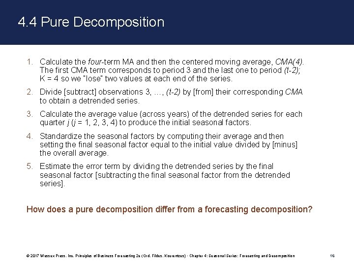
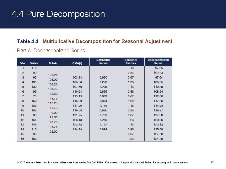
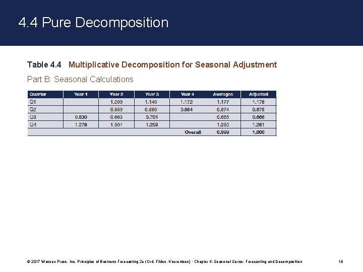
4. 4 Pure Decomposition 1. Calculate the four-term MA and then the centered moving average, CMA(4). The first CMA term corresponds to period 3 and the last one to period (t-2); K = 4 so we “lose” two values at each end of the series. 2. Divide [subtract] observations 3, …, (t-2) by [from] their corresponding CMA to obtain a detrended series. 3. Calculate the average value (across years) of the detrended series for each quarter j (j = 1, 2, 3, 4) to produce the initial seasonal factors. 4. Standardize the seasonal factors by computing their average and then setting the final seasonal factor equal to the initial value divided by [minus] the overall average. 5. Estimate the error term by dividing the detrended series by the final seasonal factor [subtracting the final seasonal factor from the detrended series]. How does a pure decomposition differ from a forecasting decomposition? © 2017 Wessex Press, Inc. Principles of Business Forecasting 2 e (Ord, Fildes, Kourentzes) • Chapter 4: Seasonal Series: Forecasting and Decomposition 16

4. 4 Pure Decomposition Table 4. 4 Multiplicative Decomposition for Seasonal Adjustment Part A: Deseasonalized Series © 2017 Wessex Press, Inc. Principles of Business Forecasting 2 e (Ord, Fildes, Kourentzes) • Chapter 4: Seasonal Series: Forecasting and Decomposition 17

4. 4 Pure Decomposition Table 4. 4 Multiplicative Decomposition for Seasonal Adjustment Part B: Seasonal Calculations © 2017 Wessex Press, Inc. Principles of Business Forecasting 2 e (Ord, Fildes, Kourentzes) • Chapter 4: Seasonal Series: Forecasting and Decomposition 18

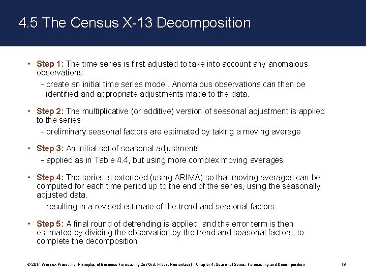
4. 5 The Census X-13 Decomposition • Step 1: The time series is first adjusted to take into account any anomalous observations –create an initial time series model. Anomalous observations can then be identified and appropriate adjustments made to the data. • Step 2: The multiplicative (or additive) version of seasonal adjustment is applied to the series –preliminary seasonal factors are estimated by taking a moving average • Step 3: An initial set of seasonal adjustments –applied as in Table 4. 4, but using more complex moving averages • Step 4: The series is extended (using ARIMA) so that moving averages can be computed for each time period up to the end of the series, using the seasonally adjusted data. –resulting in a revised estimate of the trend and seasonal factors • Step 5: A final round of detrending is applied, and the error term is then estimated by dividing the observation by the trend and seasonal factors, to complete the decomposition. © 2017 Wessex Press, Inc. Principles of Business Forecasting 2 e (Ord, Fildes, Kourentzes) • Chapter 4: Seasonal Series: Forecasting and Decomposition 19

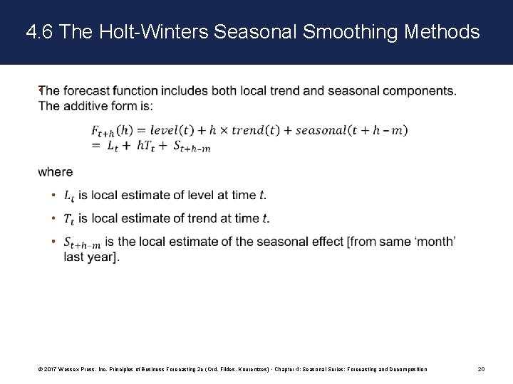
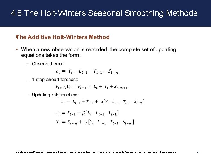
4. 6 The Holt-Winters Seasonal Smoothing Methods • © 2017 Wessex Press, Inc. Principles of Business Forecasting 2 e (Ord, Fildes, Kourentzes) • Chapter 4: Seasonal Series: Forecasting and Decomposition 20

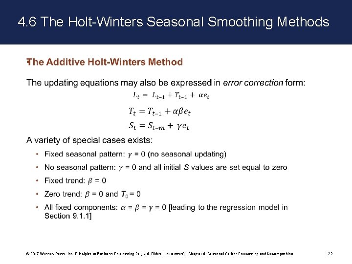
4. 6 The Holt-Winters Seasonal Smoothing Methods • © 2017 Wessex Press, Inc. Principles of Business Forecasting 2 e (Ord, Fildes, Kourentzes) • Chapter 4: Seasonal Series: Forecasting and Decomposition 21

4. 6 The Holt-Winters Seasonal Smoothing Methods • © 2017 Wessex Press, Inc. Principles of Business Forecasting 2 e (Ord, Fildes, Kourentzes) • Chapter 4: Seasonal Series: Forecasting and Decomposition 22

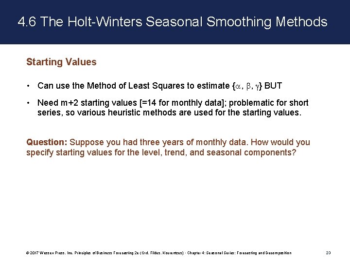
4. 6 The Holt-Winters Seasonal Smoothing Methods Starting Values • Can use the Method of Least Squares to estimate { , , } BUT • Need m+2 starting values [=14 for monthly data]; problematic for short series, so various heuristic methods are used for the starting values. Question: Suppose you had three years of monthly data. How would you specify starting values for the level, trend, and seasonal components? © 2017 Wessex Press, Inc. Principles of Business Forecasting 2 e (Ord, Fildes, Kourentzes) • Chapter 4: Seasonal Series: Forecasting and Decomposition 23

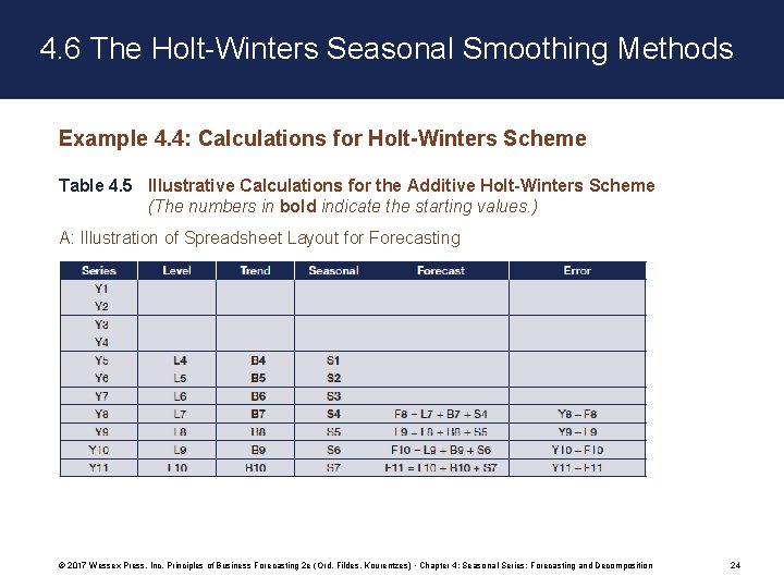
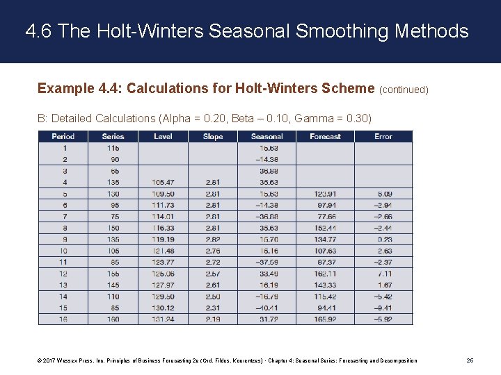
4. 6 The Holt-Winters Seasonal Smoothing Methods Example 4. 4: Calculations for Holt-Winters Scheme Table 4. 5 Illustrative Calculations for the Additive Holt-Winters Scheme (The numbers in bold indicate the starting values. ) A: Illustration of Spreadsheet Layout for Forecasting © 2017 Wessex Press, Inc. Principles of Business Forecasting 2 e (Ord, Fildes, Kourentzes) • Chapter 4: Seasonal Series: Forecasting and Decomposition 24

4. 6 The Holt-Winters Seasonal Smoothing Methods Example 4. 4: Calculations for Holt-Winters Scheme (continued) B: Detailed Calculations (Alpha = 0. 20, Beta – 0. 10, Gamma = 0. 30) © 2017 Wessex Press, Inc. Principles of Business Forecasting 2 e (Ord, Fildes, Kourentzes) • Chapter 4: Seasonal Series: Forecasting and Decomposition 25

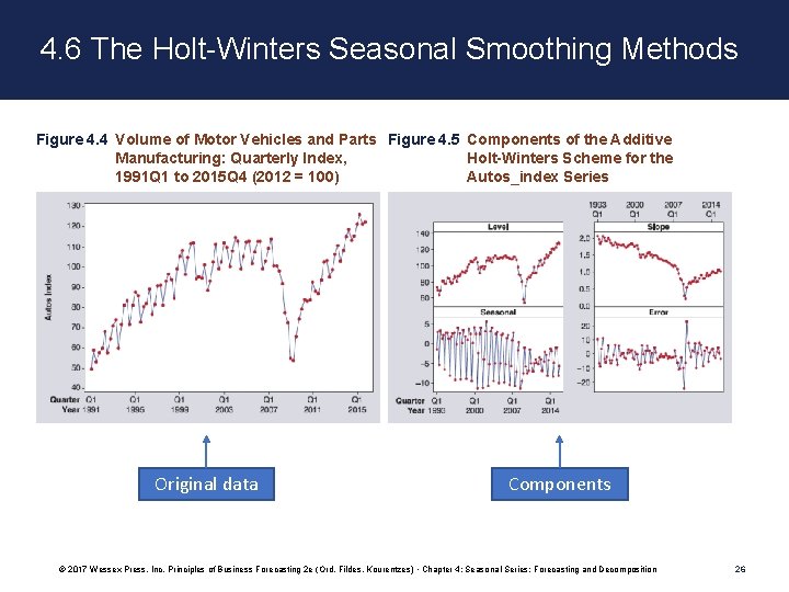
4. 6 The Holt-Winters Seasonal Smoothing Methods Figure 4. 4 Volume of Motor Vehicles and Parts Figure 4. 5 Components of the Additive Manufacturing: Quarterly Index, Holt-Winters Scheme for the 1991 Q 1 to 2015 Q 4 (2012 = 100) Autos_index Series Original data Components © 2017 Wessex Press, Inc. Principles of Business Forecasting 2 e (Ord, Fildes, Kourentzes) • Chapter 4: Seasonal Series: Forecasting and Decomposition 26

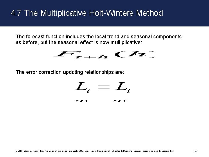
4. 7 The Multiplicative Holt-Winters Method The forecast function includes the local trend and seasonal components as before, but the seasonal effect is now multiplicative: The error correction updating relationships are: © 2017 Wessex Press, Inc. Principles of Business Forecasting 2 e (Ord, Fildes, Kourentzes) • Chapter 4: Seasonal Series: Forecasting and Decomposition 27

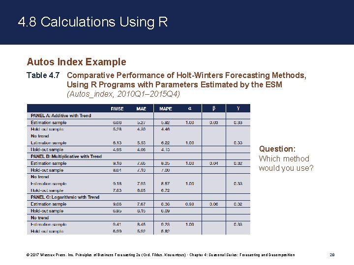
4. 8 Calculations Using R Autos Index Example Table 4. 7 Comparative Performance of Holt-Winters Forecasting Methods, Using R Programs with Parameters Estimated by the ESM (Autos_index, 2010 Q 1– 2015 Q 4) Question: Which method would you use? © 2017 Wessex Press, Inc. Principles of Business Forecasting 2 e (Ord, Fildes, Kourentzes) • Chapter 4: Seasonal Series: Forecasting and Decomposition 28

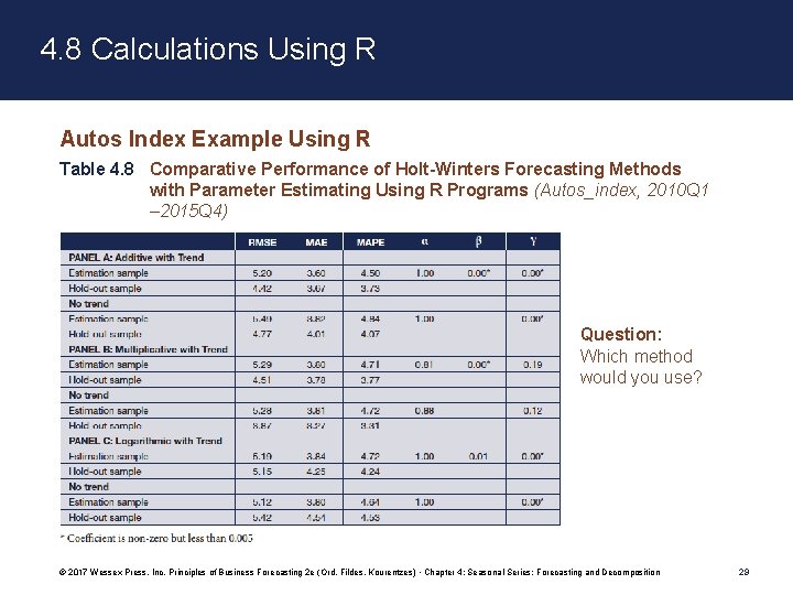
4. 8 Calculations Using R Autos Index Example Using R Table 4. 8 Comparative Performance of Holt-Winters Forecasting Methods with Parameter Estimating Using R Programs (Autos_index, 2010 Q 1 – 2015 Q 4) Question: Which method would you use? © 2017 Wessex Press, Inc. Principles of Business Forecasting 2 e (Ord, Fildes, Kourentzes) • Chapter 4: Seasonal Series: Forecasting and Decomposition 29

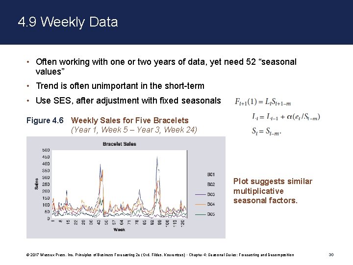
4. 9 Weekly Data • Often working with one or two years of data, yet need 52 “seasonal values” • Trend is often unimportant in the short-term • Use SES, after adjustment with fixed seasonals Figure 4. 6 Weekly Sales for Five Bracelets (Year 1, Week 5 – Year 3, Week 24) Plot suggests similar multiplicative seasonal factors. © 2017 Wessex Press, Inc. Principles of Business Forecasting 2 e (Ord, Fildes, Kourentzes) • Chapter 4: Seasonal Series: Forecasting and Decomposition 30

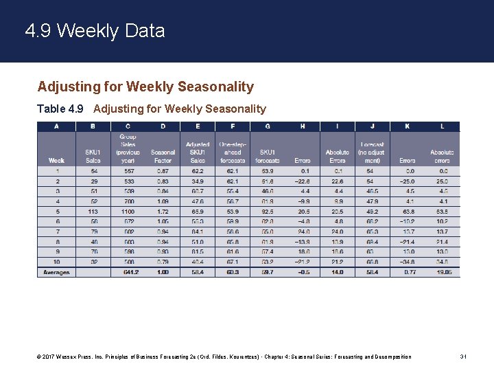
4. 9 Weekly Data Adjusting for Weekly Seasonality Table 4. 9 Adjusting for Weekly Seasonality © 2017 Wessex Press, Inc. Principles of Business Forecasting 2 e (Ord, Fildes, Kourentzes) • Chapter 4: Seasonal Series: Forecasting and Decomposition 31

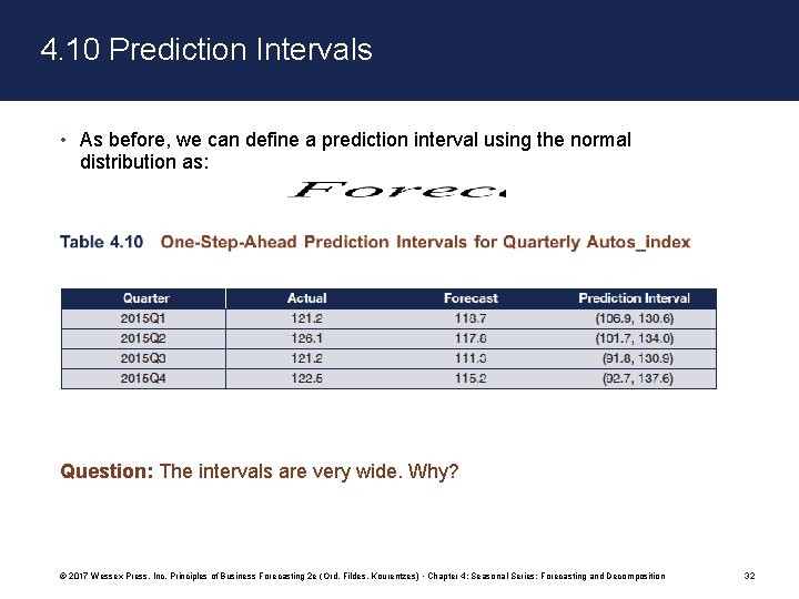
4. 10 Prediction Intervals • As before, we can define a prediction interval using the normal distribution as: Question: The intervals are very wide. Why? © 2017 Wessex Press, Inc. Principles of Business Forecasting 2 e (Ord, Fildes, Kourentzes) • Chapter 4: Seasonal Series: Forecasting and Decomposition 32

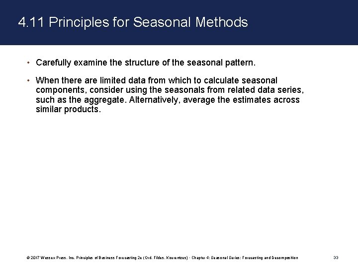
4. 11 Principles for Seasonal Methods • Carefully examine the structure of the seasonal pattern. • When there are limited data from which to calculate seasonal components, consider using the seasonals from related data series, such as the aggregate. Alternatively, average the estimates across similar products. © 2017 Wessex Press, Inc. Principles of Business Forecasting 2 e (Ord, Fildes, Kourentzes) • Chapter 4: Seasonal Series: Forecasting and Decomposition 33

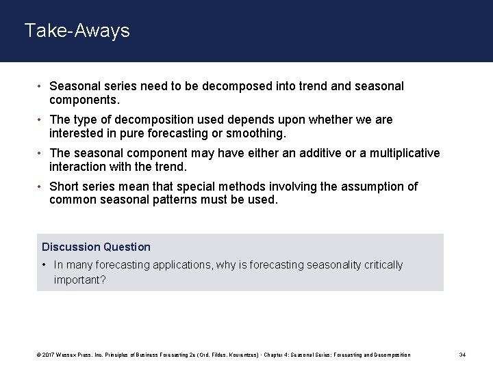
Take-Aways • Seasonal series need to be decomposed into trend and seasonal components. • The type of decomposition used depends upon whether we are interested in pure forecasting or smoothing. • The seasonal component may have either an additive or a multiplicative interaction with the trend. • Short series mean that special methods involving the assumption of common seasonal patterns must be used. Discussion Question • In many forecasting applications, why is forecasting seasonality critically important? © 2017 Wessex Press, Inc. Principles of Business Forecasting 2 e (Ord, Fildes, Kourentzes) • Chapter 4: Seasonal Series: Forecasting and Decomposition 34

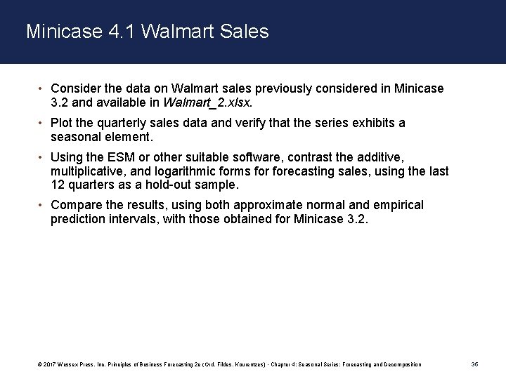
Minicase 4. 1 Walmart Sales • Consider the data on Walmart sales previously considered in Minicase 3. 2 and available in Walmart_2. xlsx. • Plot the quarterly sales data and verify that the series exhibits a seasonal element. • Using the ESM or other suitable software, contrast the additive, multiplicative, and logarithmic forms forecasting sales, using the last 12 quarters as a hold-out sample. • Compare the results, using both approximate normal and empirical prediction intervals, with those obtained for Minicase 3. 2. © 2017 Wessex Press, Inc. Principles of Business Forecasting 2 e (Ord, Fildes, Kourentzes) • Chapter 4: Seasonal Series: Forecasting and Decomposition 35

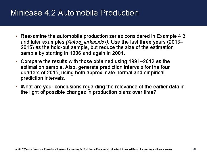
Minicase 4. 2 Automobile Production • Reexamine the automobile production series considered in Example 4. 3 and later examples (Autos_index. xlsx). Use the last three years (2013– 2015) as the hold-out sample, but reduce the size of the estimation sample by starting in 1996 and again in 2001. • Compare the results with those obtained using 1991– 2012 as the estimation sample. Also, generate prediction intervals for the four quarters of 2015, using both approximate normal and empirical prediction intervals. • What are your conclusions regarding the relevance of the earlier data in the light of possible changes in production plans over time? © 2017 Wessex Press, Inc. Principles of Business Forecasting 2 e (Ord, Fildes, Kourentzes) • Chapter 4: Seasonal Series: Forecasting and Decomposition 36

Minicase 4. 3 U. S. Retail Sales The spreadsheet US_retail_sales_2. xlsx contains the monthly values of U. S. retail sales (measured in $billions) over the period from January 2001 to December 2016. The series was plotted in Chapter 1. The spreadsheet includes the value of sales (Sales), the seasonally adjusted values (Sales_SA) and the seasonal factors. • Compare the options of: – forecasting the series by using the Holt-Winters approach, – forecasting the components separately and then combining them. • Use the period January 2001–November 2007 as the estimation sample. The onset of the "Great Recession" was determined to have occurred in December 2007 but was not officially confirmed until December 2008; would the one-step-ahead forecasts have provided earlier warning? Generate prediction intervals and see whether the actual values fall within the limits. • If you have access to suitable software, evaluate the ability of the multiple-step-ahead forecasts to predict the downturn. Conduct a rolling origin 1 -12 evaluation, forecasting for the years 2008– 2010. (If no suitable software is available, use just three forecast origins to compare results. ) • Extend the estimation sample to December 2012 and compare the one-step-ahead forecast performance for the period 2013– 2015 using the two different estimation samples. [Exercise 4. 6] © 2017 Wessex Press, Inc. Principles of Business Forecasting 2 e (Ord, Fildes, Kourentzes) • Chapter 4: Seasonal Series: Forecasting and Decomposition 37

Minicase 4. 4 UK Retail Sales The spreadsheet UK_retail_sales_2. xlsx contains the quarterly values of the UK Retail Sales Index (measured with 2010 set at 100), both unadjusted and seasonally adjusted, over the period from January 1996 to December 2014. • Create a purely seasonal series by dividing the unadjusted series by the seasonally adjusted one. Using one-step-ahead forecasts, compare the options of: – Forecasting the series by using the Holt-Winters approach. – Forecasting the components separately and then combining them. It is recommended that you use the period 1996– 2011 for estimation and the remaining 12 quarters as the hold-out sample. © 2017 Wessex Press, Inc. Principles of Business Forecasting 2 e (Ord, Fildes, Kourentzes) • Chapter 4: Seasonal Series: Forecasting and Decomposition 38

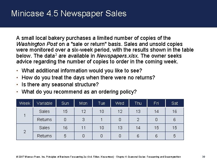
Minicase 4. 5 Newspaper Sales A small local bakery purchases a limited number of copies of the Washington Post on a "sale or return" basis. Sales and unsold copies were monitored over a six-week period, with the results shown in the table below. The data 3 are available in Newspapers. xlsx. The owner seeks advice regarding the number of copies to order in the coming week. • • What additional information would you like to see? How do you treat the days when there were no returns? Is there any seasonal structure? What do you recommend as an ordering policy? Week 1 2 Variable Sun Mon Tue Wed Thu Fri Sat Sales 15 12 10 12 13 14 16 Returns 0 3 1 0 2 0 6 Sales 16 11 10 13 14 15 15 Returns 5 0 0 0 6 6 5 © 2017 Wessex Press, Inc. Principles of Business Forecasting 2 e (Ord, Fildes, Kourentzes) • Chapter 4: Seasonal Series: Forecasting and Decomposition 39