CHAPTER 3 Forecasting Jihan Sheikh Ahmad Kulliyyah of

CHAPTER 3 Forecasting Jihan Sheikh Ahmad Kulliyyah of Muamalat, Insaniah University College

What is Forecasting? FORECAST: • A statement about the future value of a variable of interest such as demand. • Forecasts affect decisions and activities throughout an organization – Accounting, finance – Human resources – Marketing – MIS – Operations – Product / service design

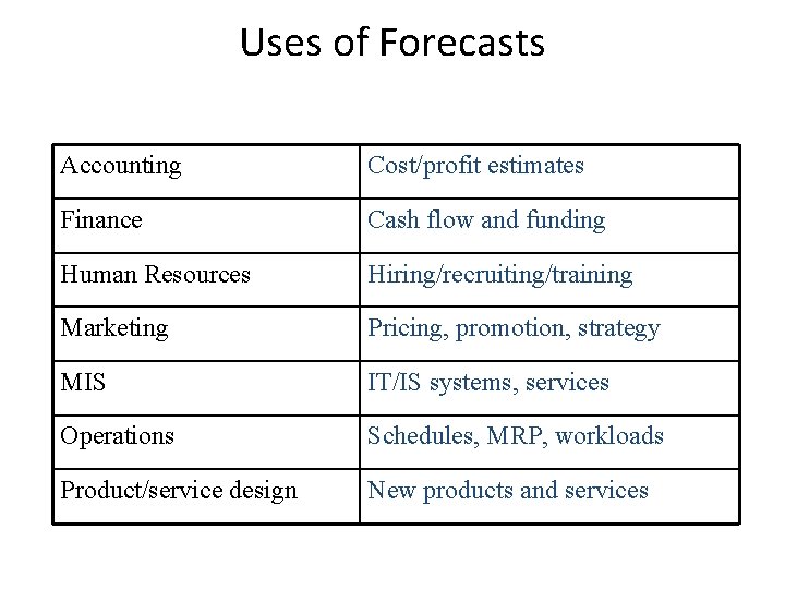
Uses of Forecasts Accounting Cost/profit estimates Finance Cash flow and funding Human Resources Hiring/recruiting/training Marketing Pricing, promotion, strategy MIS IT/IS systems, services Operations Schedules, MRP, workloads Product/service design New products and services

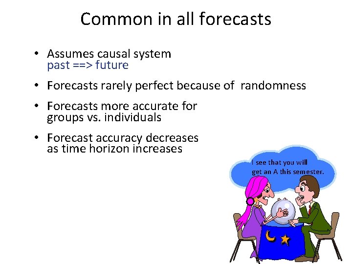
Common in all forecasts • Assumes causal system past ==> future • Forecasts rarely perfect because of randomness • Forecasts more accurate for groups vs. individuals • Forecast accuracy decreases as time horizon increases I see that you will get an A this semester.

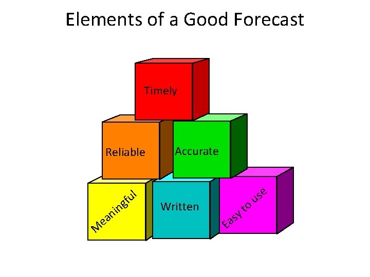
Elements of a Good Forecast Timely Reliable g l fu M in n ea Accurate Written s a E o t y e s u

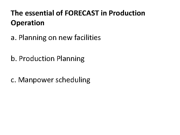
The essential of FORECAST in Production Operation a. Planning on new facilities b. Production Planning c. Manpower scheduling

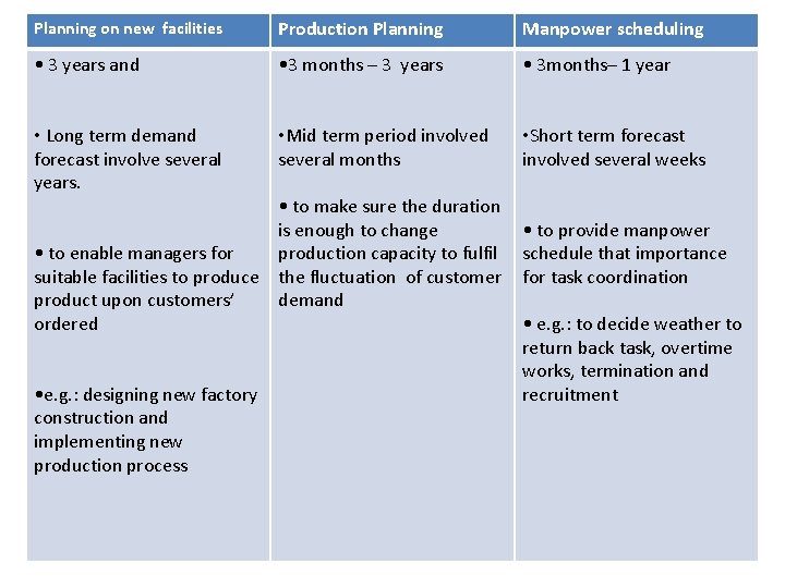
Planning on new facilities Production Planning Manpower scheduling • 3 years and • 3 months – 3 years • 3 months– 1 year • Long term demand forecast involve several years. • Mid term period involved several months • Short term forecast involved several weeks • to make sure the duration is enough to change • to enable managers for production capacity to fulfil suitable facilities to produce the fluctuation of customer product upon customers’ demand ordered • e. g. : designing new factory construction and implementing new production process • to provide manpower schedule that importance for task coordination • e. g. : to decide weather to return back task, overtime works, termination and recruitment

Time Horizon • Short term • Medium term • Long term

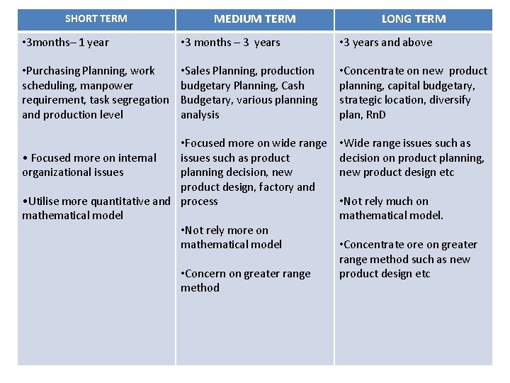
SHORT TERM MEDIUM TERM LONG TERM • 3 months– 1 year • 3 months – 3 years • 3 years and above • Purchasing Planning, work scheduling, manpower requirement, task segregation and production level • Sales Planning, production budgetary Planning, Cash Budgetary, various planning analysis • Concentrate on new product planning, capital budgetary, strategic location, diversify plan, Rn. D • Focused more on wide range • Focused more on internal issues such as product organizational issues planning decision, new product design, factory and • Utilise more quantitative and process mathematical model • Not rely more on mathematical model • Concern on greater range method • Wide range issues such as decision on product planning, new product design etc • Not rely much on mathematical model. • Concentrate ore on greater range method such as new product design etc

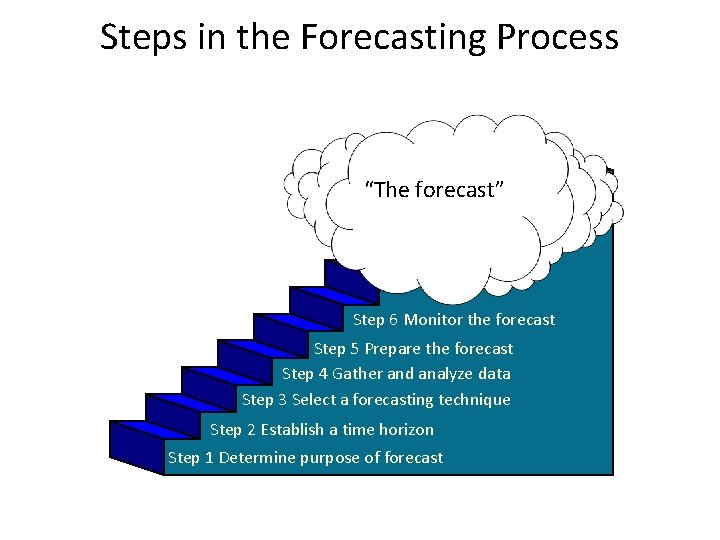
Steps in the Forecasting Process “The forecast” Step 6 Monitor the forecast Step 5 Prepare the forecast Step 4 Gather and analyze data Step 3 Select a forecasting technique Step 2 Establish a time horizon Step 1 Determine purpose of forecast

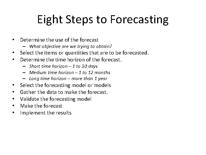
Eight Steps to Forecasting • Determine the use of the forecast – What objective are we trying to obtain? • Select the items or quantities that are to be forecasted. • Determine the time horizon of the forecast. – Short time horizon – 1 to 30 days – Medium time horizon – 1 to 12 months – Long time horizon – more than 1 year • • • Select the forecasting model or models Gather the data to make the forecast. Validate the forecasting model Make the forecast Implement the results

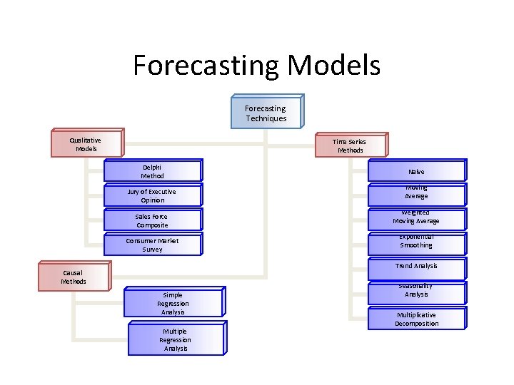
Forecasting Models Forecasting Techniques Qualitative Models Time Series Methods Delphi Method Jury of Executive Opinion Sales Force Composite Consumer Market Survey Naive Moving Average Weighted Moving Average Exponential Smoothing Trend Analysis Causal Methods Simple Regression Analysis Multiple Regression Analysis Seasonality Analysis Multiplicative Decomposition

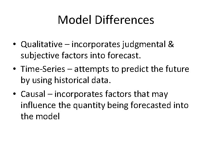
Model Differences • Qualitative – incorporates judgmental & subjective factors into forecast. • Time-Series – attempts to predict the future by using historical data. • Causal – incorporates factors that may influence the quantity being forecasted into the model

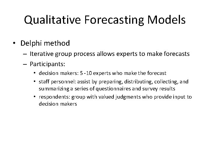
Qualitative Forecasting Models • Delphi method – Iterative group process allows experts to make forecasts – Participants: • decision makers: 5 -10 experts who make the forecast • staff personnel: assist by preparing, distributing, collecting, and summarizing a series of questionnaires and survey results • respondents: group with valued judgments who provide input to decision makers

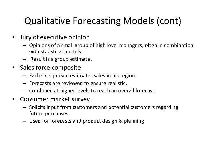
Qualitative Forecasting Models (cont) • Jury of executive opinion – Opinions of a small group of high level managers, often in combination with statistical models. – Result is a group estimate. • Sales force composite – Each salesperson estimates sales in his region. – Forecasts are reviewed to ensure realistic. – Combined at higher levels to reach an overall forecast. • Consumer market survey. – Solicits input from customers and potential customers regarding future purchases. – Used forecasts and product design & planning

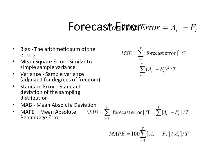
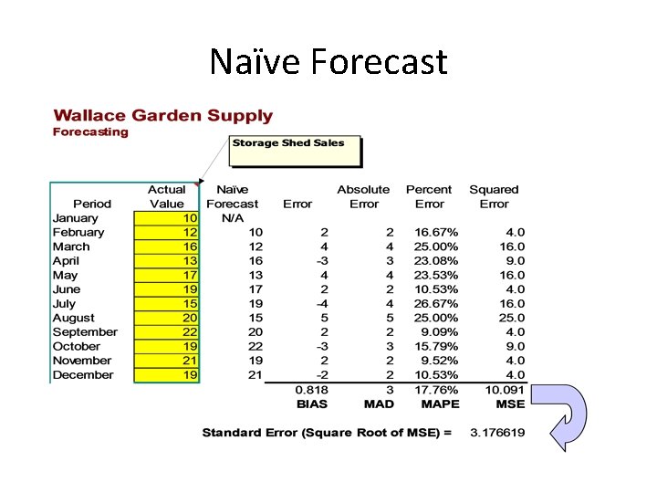
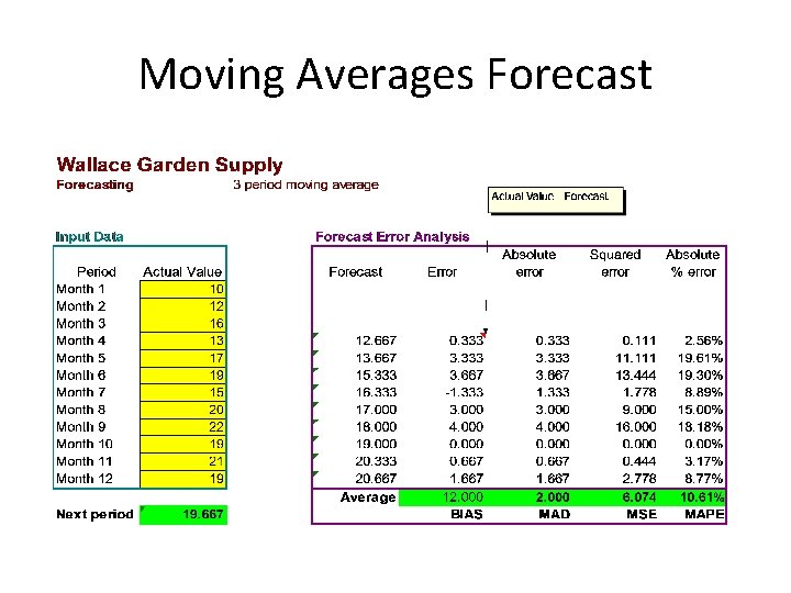
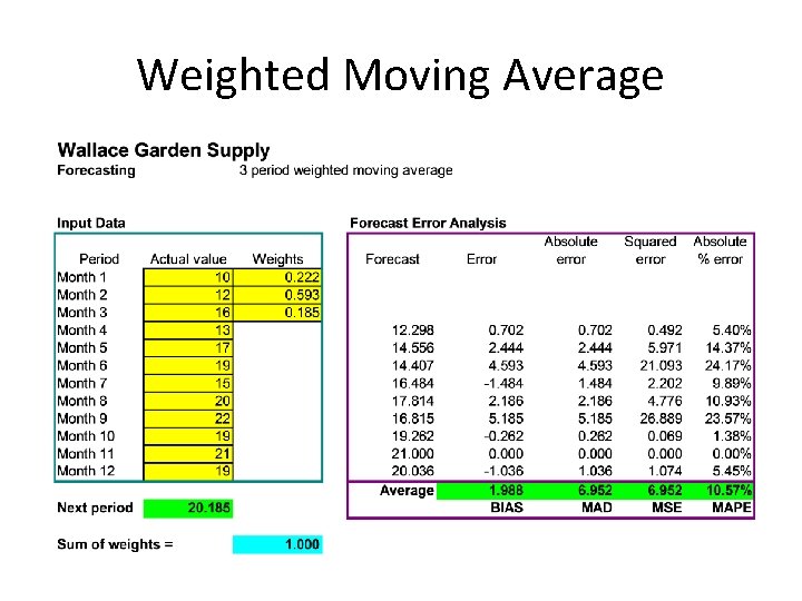
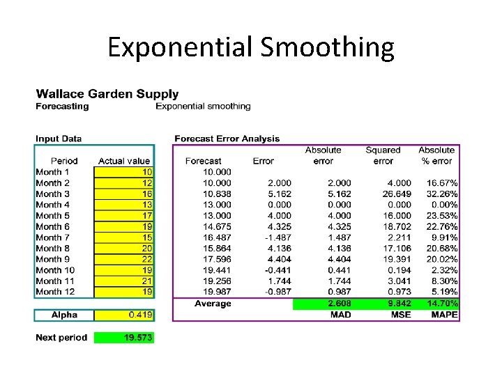
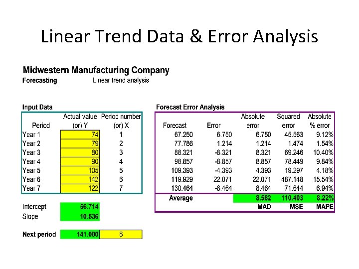
Forecast Error • Bias - The arithmetic sum of the errors • Mean Square Error - Similar to simple sample variance • Variance - Sample variance (adjusted for degrees of freedom) • Standard Error - Standard deviation of the sampling distribution • MAD - Mean Absolute Deviation • MAPE – Mean Absolute Percentage Error

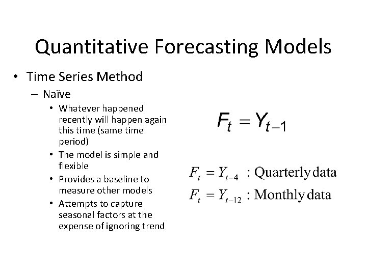
Quantitative Forecasting Models • Time Series Method – Naïve • Whatever happened recently will happen again this time (same time period) • The model is simple and flexible • Provides a baseline to measure other models • Attempts to capture seasonal factors at the expense of ignoring trend

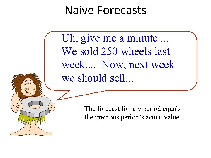
Naive Forecasts Uh, give me a minute. . We sold 250 wheels last week. . Now, next week we should sell. . The forecast for any period equals the previous period’s actual value.

Naïve Forecast

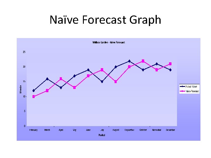
Naïve Forecast Graph

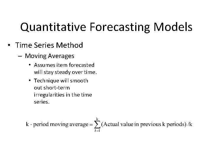
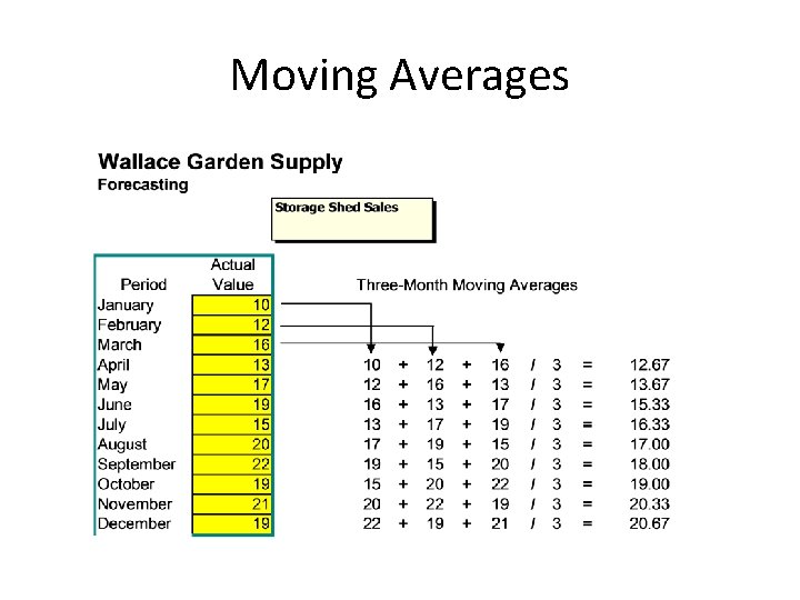
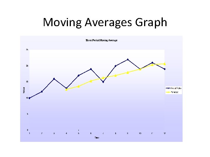
Quantitative Forecasting Models • Time Series Method – Moving Averages • Assumes item forecasted will stay steady over time. • Technique will smooth out short-term irregularities in the time series.

Moving Averages

Moving Averages Forecast

Moving Averages Graph

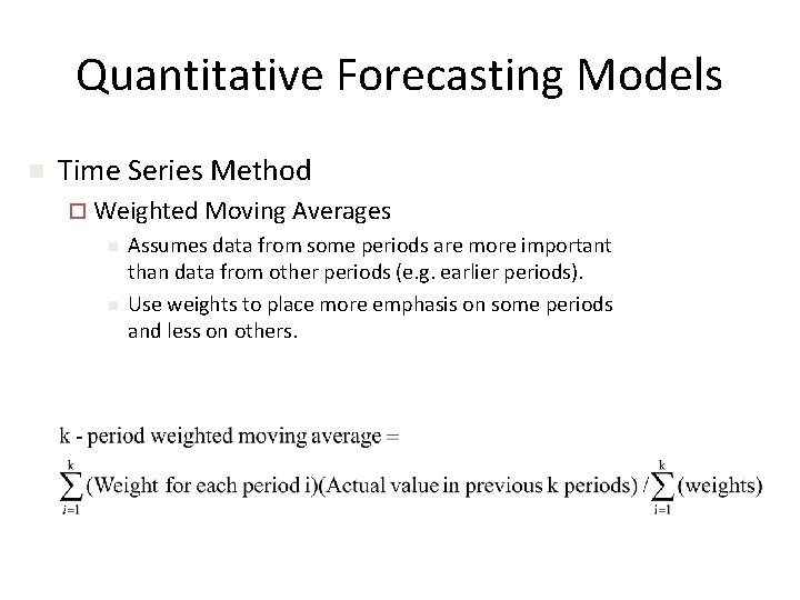
Quantitative Forecasting Models n Time Series Method ¨ Weighted Moving Averages n n Assumes data from some periods are more important than data from other periods (e. g. earlier periods). Use weights to place more emphasis on some periods and less on others.

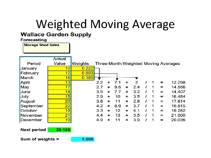
Weighted Moving Average

Weighted Moving Average

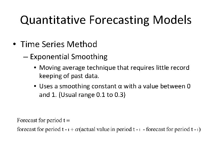
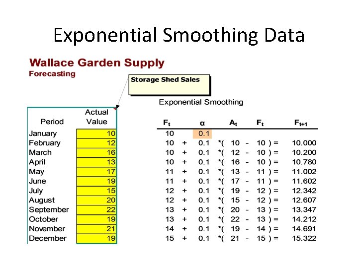
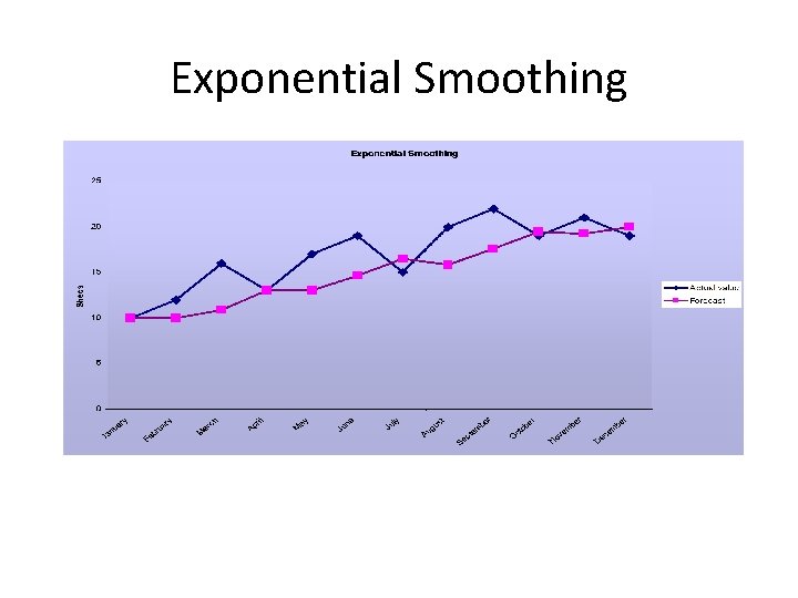
Quantitative Forecasting Models • Time Series Method – Exponential Smoothing • Moving average technique that requires little record keeping of past data. • Uses a smoothing constant α with a value between 0 and 1. (Usual range 0. 1 to 0. 3)

Exponential Smoothing Data

Exponential Smoothing

Exponential Smoothing

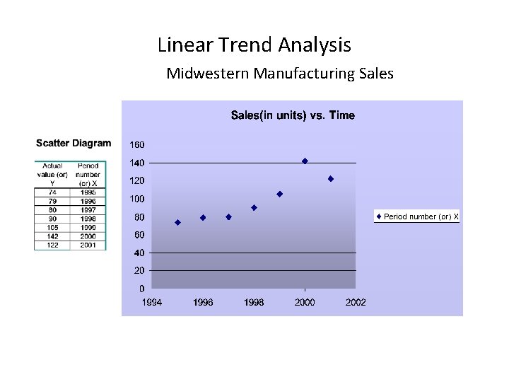
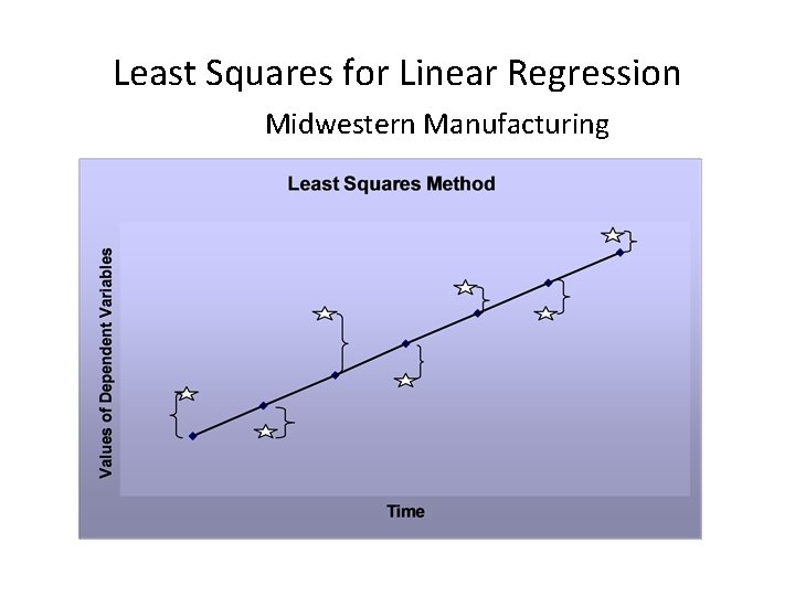
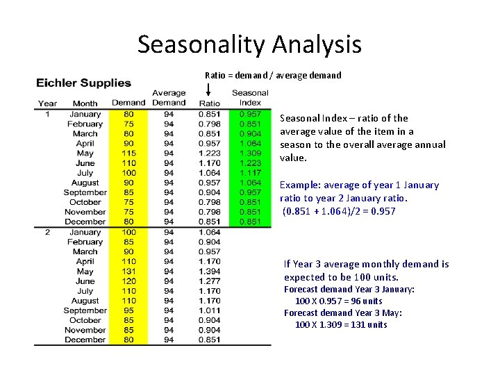
Trend & Seasonality • Trend analysis – technique that fits a trend equation (or curve) to a series of historical data points. – projects the curve into the future for medium and long term forecasts. • Seasonality analysis – adjustment to time series data due to variations at certain periods. – adjust with seasonal index – ratio of average value of the item in a season to the overall annual average value. – example: demand for coal & fuel oil in winter months.

Linear Trend Analysis Midwestern Manufacturing Sales

Least Squares for Linear Regression Midwestern Manufacturing

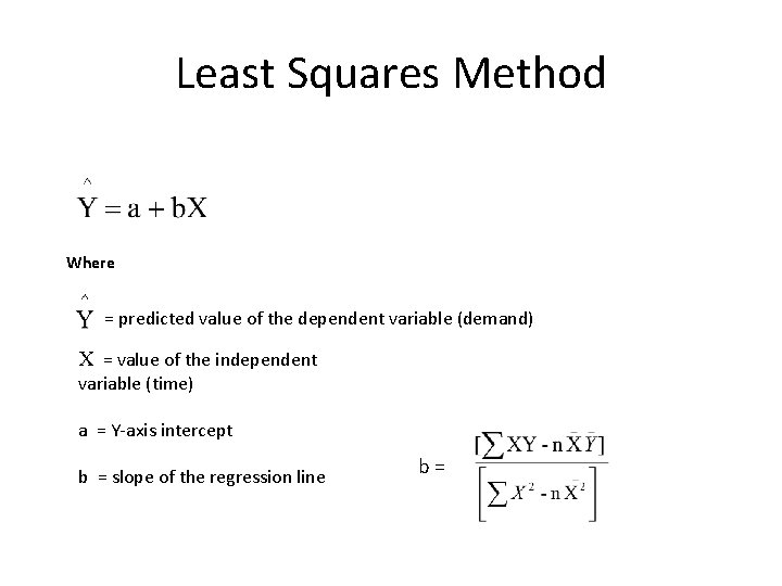
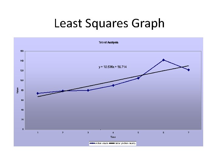
Least Squares Method Where = predicted value of the dependent variable (demand) X = value of the independent variable (time) a = Y-axis intercept b = slope of the regression line b=

Linear Trend Data & Error Analysis

Least Squares Graph

Seasonality Analysis Ratio = demand / average demand Seasonal Index – ratio of the average value of the item in a season to the overall average annual value. Example: average of year 1 January ratio to year 2 January ratio. (0. 851 + 1. 064)/2 = 0. 957 If Year 3 average monthly demand is expected to be 100 units. Forecast demand Year 3 January: 100 X 0. 957 = 96 units Forecast demand Year 3 May: 100 X 1. 309 = 131 units

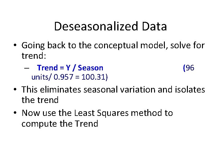
Deseasonalized Data • Going back to the conceptual model, solve for trend: – Trend = Y / Season units/ 0. 957 = 100. 31) (96 • This eliminates seasonal variation and isolates the trend • Now use the Least Squares method to compute the Trend

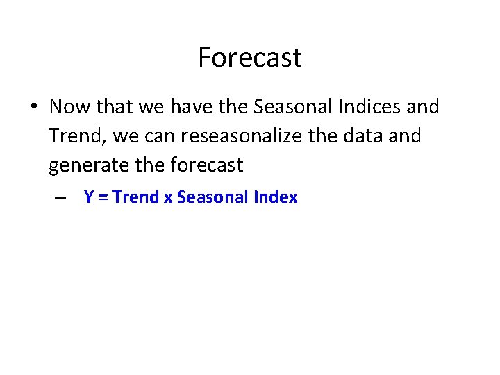
Forecast • Now that we have the Seasonal Indices and Trend, we can reseasonalize the data and generate the forecast – Y = Trend x Seasonal Index