Chapter 19 Confidence Intervals for Proportions Copyright 2009

Standard Deviation of Sampling Distribution n Both of the sampling distributions we’ve looked at

Standard Error n n n When we don’t know p or σ, we’re stuck,

Standard Error n For a sample proportion, the standard error is n For the

A Confidence Interval n Recall that the sampling distribution model of centered at p,

A Confidence Interval (cont. ) n n By the 68 -95 -99. 7% Rule,

A Confidence Interval (cont. ) n n Consider the 95% level: n There’s a

A Confidence Interval (cont. ) Copyright © 2009 Pearson Education, Inc. Slide 1 -

What Does “ 95% Confidence” Really Mean? n n Each confidence interval uses a

What Does “ 95% Confidence” Really Mean? n The figure to the right shows

What Does “ 95% Confidence” Really Mean? n n Our confidence is in the

Margin of Error: Certainty vs. Precision n We can claim, with 95% confidence, that

Margin of Error: Certainty vs. Precision Copyright © 2009 Pearson Education, Inc. Slide 1

Margin of Error: Certainty vs. Precision n To be more confident, we wind up

Margin of Error: Certainty vs. Precision n n The choice of confidence level is

Critical Values n n n The ‘ 2’ in (our 95% confidence interval) came

Critical Values (cont. ) n Example: For a 90% confidence interval, the critical value

One-Proportion (z) Interval n n When the conditions are met, we are ready to

Universal Conditions (Formulas) 1. Randomization Condition: The sample should be a simple random sample

1 -Proportion • Categorical Data • You use p-hat and q-hat to approximate the

Steps for Constructing and Interpreting a Confidence Interval 1) 2) 3) 4) 5) 6)

Writing your interpretation We are (___)% confident that the (mean or proportion of…. (in

Copyright © 2009 Pearson Education, Inc. Slide 1 - 23

Copyright © 2009 Pearson Education, Inc. Slide 1 - 24

Copyright © 2009 Pearson Education, Inc. Slide 1 - 25

Copyright © 2009 Pearson Education, Inc. Slide 1 - 26

Confidence Intervals for a Population Mean (Quantitative) z vs. t distributions • • •

Sample means “Quantitative” z vs. t Z intervals are for when sigma (SD of

1 -Sample Z-test • Quantitative Data • You know (sigma) the standard deviation of

1 -Sample t-test • Quantitative Data • You do not know (sigma) the standard

Standardize using s for n Substitute s (sample standard deviation) for sssssss s Note

t-distributions Suppose that a Simple Random Sample of size n is drawn from a

Confidence Interval Estimates n CONFIDENCE INTERVAL for n n n n where: t =

Student’s t Distribution Z -3 -3 -2 -2 -1 -1 00 11 22 33

Student’s t Distribution Z t -3 -3 -2 -2 -1 -1 00 11 22

n Example – An investor is trying to estimate the return on investment in

Example n n n Because cardiac deaths increase after heavy snowfalls, a study was

EXAMPLE: Consumer Protection Agency n n Selected random sample of 16 packages of a

Choosing type of Interval n n n Categorical Data: 1 -Proportion (Z) Interval *NO

Slides: 42

Download presentation

Standard Error n n n When we don’t know p or σ, we’re stuck, right? Nope. We will use sample statistics to estimate these population parameters. Whenever we estimate the standard deviation of a sampling distribution, we call it a standard error. Copyright © 2009 Pearson Education, Inc. Slide 1 - 3

A Confidence Interval n Recall that the sampling distribution model of centered at p, with standard deviation n is. Since we don’t know p, we can’t find the true standard deviation of the sampling distribution model, so we need to find the standard error: Copyright © 2009 Pearson Education, Inc. Slide 1 - 5

A Confidence Interval (cont. ) n n By the 68 -95 -99. 7% Rule, we know n about 68% of all samples will have ’s within 1 SE of p n about 95% of all samples will have ’s within 2 SEs of p n about 99. 7% of all samples will have ’s within 3 SEs of p We can look at this from Copyright © 2009 Pearson Education, Inc. ’s point of view… Slide 1 - 6

A Confidence Interval (cont. ) n n Consider the 95% level: n There’s a 95% chance that p is no more than 2 SEs away from. n So, if we reach out 2 SEs, we are 95% sure that p will be in that interval. In other words, if we reach out 2 SEs in either direction of , we can be 95% confident that this interval contains the true proportion. This is called a 95% confidence interval. Copyright © 2009 Pearson Education, Inc. Slide 1 - 7

What Does “ 95% Confidence” Really Mean? n n Each confidence interval uses a sample statistic to estimate a population parameter. But, since samples vary, the statistics we use, and thus the confidence intervals we construct, vary as well. Copyright © 2009 Pearson Education, Inc. Slide 1 - 9

What Does “ 95% Confidence” Really Mean? n The figure to the right shows that some of our confidence intervals (from 20 random samples) capture the true proportion (the green horizontal line), while others do not: Copyright © 2009 Pearson Education, Inc. Slide 1 - 10

What Does “ 95% Confidence” Really Mean? n n Our confidence is in the process of constructing the interval, not in any one interval itself. Thus, we expect 95% of all 95% confidence intervals to contain the true parameter that they are estimating. Copyright © 2009 Pearson Education, Inc. Slide 1 - 11

Margin of Error: Certainty vs. Precision n We can claim, with 95% confidence, that the interval contains the true population proportion. n The extent of the interval on either side of is called the margin of error (ME). In general, confidence intervals have the form estimate ± ME. The more confident we want to be, the larger our ME needs to be (makes the interval wider). Slide 1 - 12 Copyright © 2009 Pearson Education, Inc.

Margin of Error: Certainty vs. Precision n To be more confident, we wind up being less precise. n We need more values in our confidence interval to be more certain. Because of this, every confidence interval is a balance between certainty and precision. The tension between certainty and precision is always there. n Fortunately, in most cases we can be both sufficiently certain and sufficiently precise to make useful statements. Copyright © 2009 Pearson Education, Inc. Slide 1 - 14

Margin of Error: Certainty vs. Precision n n The choice of confidence level is somewhat arbitrary, but keep in mind this tension between certainty and precision when selecting your confidence level. The most commonly chosen confidence levels are 90%, 95%, and 99% (but any percentage can be used). Copyright © 2009 Pearson Education, Inc. Slide 1 - 15

Critical Values n n n The ‘ 2’ in (our 95% confidence interval) came from the 68 -95 -99. 7% Rule. Using a table or technology, we find that a more exact value for our 95% confidence interval is 1. 96 instead of 2. n We call 1. 96 the critical value and denote it z*. For any confidence level, we can find the corresponding critical value. Copyright © 2009 Pearson Education, Inc. Slide 1 - 16

One-Proportion (z) Interval n n When the conditions are met, we are ready to find the confidence interval for the population proportion, p. The confidence interval is where n The critical value, z*, depends on the particular confidence level, C, that you specify. Copyright © 2009 Pearson Education, Inc. Slide 1 - 18

Universal Conditions (Formulas) 1. Randomization Condition: The sample should be a simple random sample of the population. 2. 10% Condition: (Independence) If sampling has not been made with replacement, and you are drawing from a finite population the sample size, n, must be no larger than 10% of the population. (10 n < Pop. Size)

1 -Proportion • Categorical Data • You use p-hat and q-hat to approximate the standard deviation of the population. • Normality Check: The sample size has to be big enough so that both np and n(1 -p) are at least 10.

Steps for Constructing and Interpreting a Confidence Interval 1) 2) 3) 4) 5) 6) State your population (NOT the sample) State the parameter of interest (Mu or p) State the Type of Interval (1 -prop, 1 -samp Z, or 1 -samp t) Check Conditions (If Needed) Show symbols and values and calculate interval on Stat Crunch. Interpret the Interval. Copyright © 2009 Pearson Education, Inc. Slide 1 - 21

Confidence Intervals for a Population Mean (Quantitative) z vs. t distributions • • • z and t distributions Z and t confidence intervals for a population mean Sample size required to estimate

Sample means “Quantitative” z vs. t Z intervals are for when sigma (SD of the population) is known. n T intervals are for when sigma (SD of the population) is unknown and we use “s” (SD of the sample) to approximate sigma. n

1 -Sample Z-test • Quantitative Data • You know (sigma) the standard deviation of the population. • Normality Check: Stated in the question, probability plot, n is at least 30.

1 -Sample t-test • Quantitative Data • You do not know (sigma) the standard deviation of the population. • You use “s” the standard deviation of the sample to approximate sigma. • Normality Check: (Central Limit Theorem) Sample Size of at least 30

Standardize using s for n Substitute s (sample standard deviation) for sssssss s Note quite correct Not knowing means using z is no longer correct

t-distributions Suppose that a Simple Random Sample of size n is drawn from a population whose distribution can be approximated by a N(µ, σ) model. When is known, the sampling model for the mean x is N( , /√n), so is approximately Z~N(0, 1). When is estimated from the sample standard deviation s, the sampling model for follows a t distribution with degrees of freedom n − 1. is the 1 -sample t statistic

Confidence Interval Estimates n CONFIDENCE INTERVAL for n n n n where: t = Critical value from -distribution with n-1 degrees of freedom = Sample mean s = Sample standard deviation n = Sample size t For small samples (n < 30), the data should follow a Normal model very closely. For sample sizes larger than 30, t methods are safe to use.

Student’s t Distribution Z -3 -3 -2 -2 -1 -1 00 11 22 33

Student’s t Distribution Z t -3 -3 -2 -2 -1 -1 00 11 22 33 Figure 11. 3, Page 372

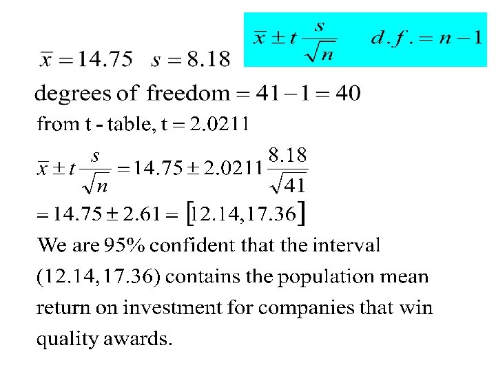
n Example – An investor is trying to estimate the return on investment in companies that won quality awards last year. – A random sample of 41 such companies is selected, and the return on investment is recorded for each company. The data for the 41 companies have – Construct a 95% confidence interval for the mean return.

Example n n n Because cardiac deaths increase after heavy snowfalls, a study was conducted to measure the cardiac demands of shoveling snow by hand The maximum heart rates for 10 adult males were recorded while shoveling snow. The sample mean and sample standard deviation were Assuming the distribution is Normal, find a 90% CI for the population mean max. heart rate for those who shovel snow.

Solution

EXAMPLE: Consumer Protection Agency n n Selected random sample of 16 packages of a product whose packages are marked as weighing 1 pound. From the 16 packages: a. find a 95% CI for the mean weight of the 1 -pound packages n b. should the company’s claim that the mean weight is 1 pound be challenged ? n

EXAMPLE

Choosing type of Interval n n n Categorical Data: 1 -Proportion (Z) Interval *NO SD is ever given Quantitative Data: 1 -Sample Z Interval *used when we know sigma (the SD of the population) Quantitative Data: 1 -Sample T Interval *used when we ONLY know the standard deviation of the sample (s) Copyright © 2009 Pearson Education, Inc. Slide 1 - 42