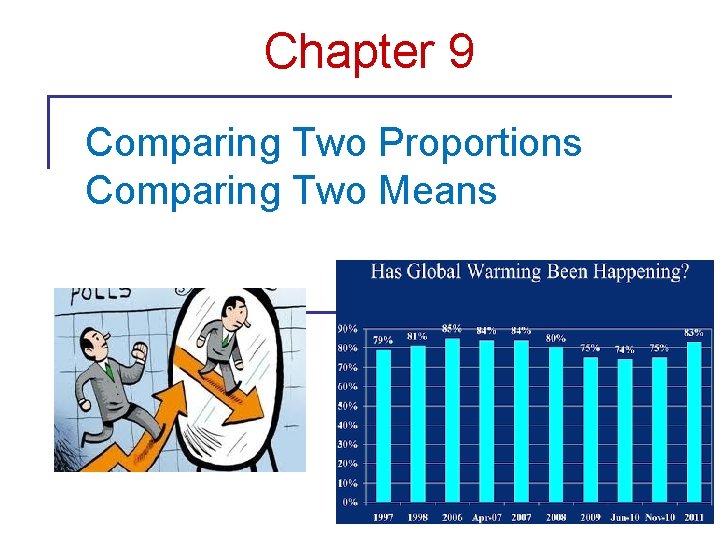
Chapter 9 Comparing Two Proportions Comparing Two Means

Chapter 9 Comparing Two Proportions Comparing Two Means © 2006 W. H. Freeman and Company

Objectives (Chapter 9) Comparing two proportions and two means p Comparing two independent samples p Large-sample CI for two proportions p CI for two means p Test of statistical significance

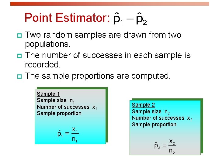
Point Estimator: p p p Two random samples are drawn from two populations. The number of successes in each sample is recorded. The sample proportions are computed. Sample 1 Sample size n 1 Number of successes x 1 Sample proportion pˆ 1 = x 1 n 1 Sample 2 Sample size n 2 Number of successes x 2 Sample proportion 3

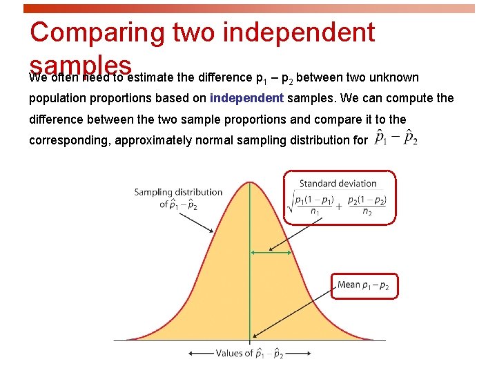
Comparing two independent samples We often need to estimate the difference p – p between two unknown 1 2 population proportions based on independent samples. We can compute the difference between the two sample proportions and compare it to the corresponding, approximately normal sampling distribution for

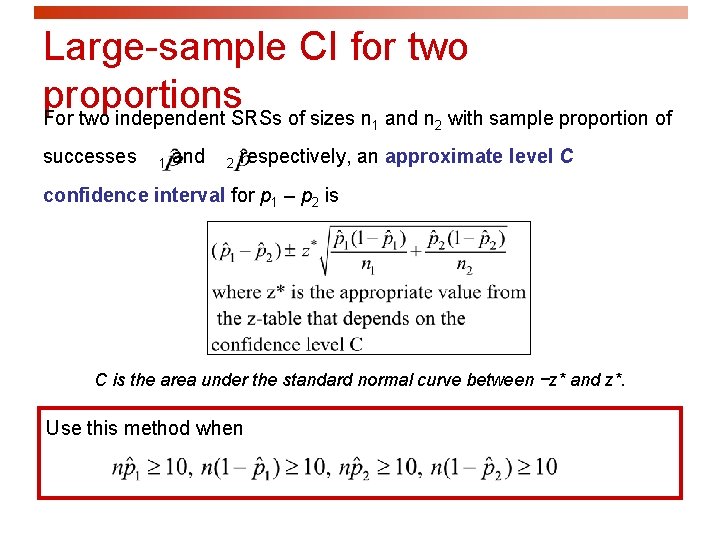
Large-sample CI for two proportions For two independent SRSs of sizes n and n with sample proportion of 1 successes 1 and 2 2 respectively, an approximate level C confidence interval for p 1 – p 2 is C is the area under the standard normal curve between −z* and z*. Use this method when

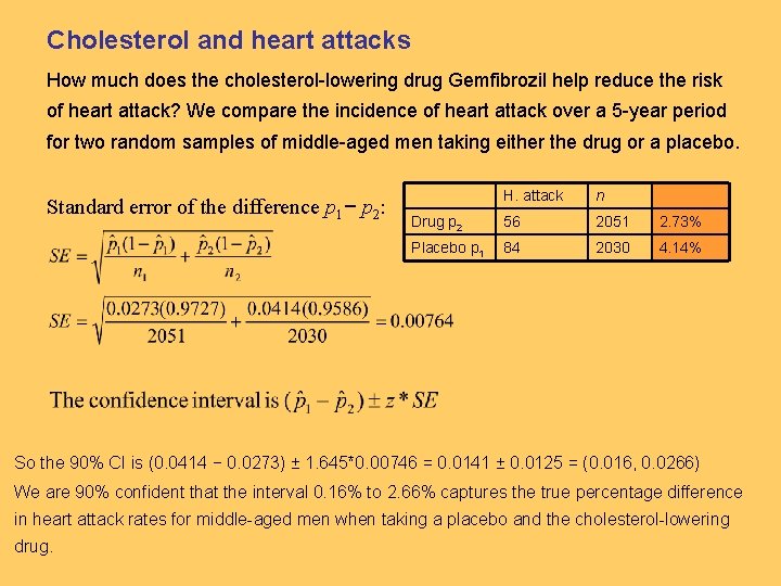
Cholesterol and heart attacks How much does the cholesterol-lowering drug Gemfibrozil help reduce the risk of heart attack? We compare the incidence of heart attack over a 5 -year period for two random samples of middle-aged men taking either the drug or a placebo. Standard error of the difference p 1− p 2: H. attack n Drug p 2 56 2051 2. 73% Placebo p 1 84 2030 4. 14% So the 90% CI is (0. 0414 − 0. 0273) ± 1. 645*0. 00746 = 0. 0141 ± 0. 0125 = (0. 016, 0. 0266) We are 90% confident that the interval 0. 16% to 2. 66% captures the true percentage difference in heart attack rates for middle-aged men when taking a placebo and the cholesterol-lowering drug.

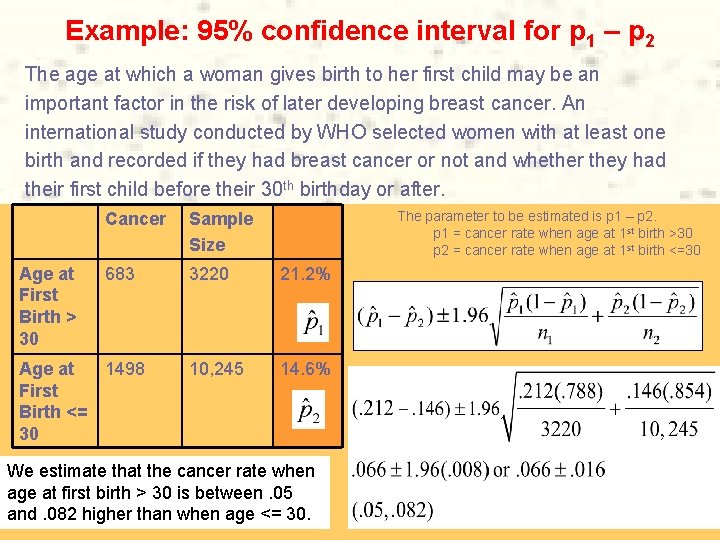
Example: 95% confidence interval for p 1 – p 2 The age at which a woman gives birth to her first child may be an important factor in the risk of later developing breast cancer. An international study conducted by WHO selected women with at least one birth and recorded if they had breast cancer or not and whether they had their first child before their 30 th birthday or after. Age at First Birth > 30 The parameter to be estimated is p 1 – p 2. p 1 = cancer rate when age at 1 st birth >30 p 2 = cancer rate when age at 1 st birth <=30 Cancer Sample Size 683 3220 21. 2% 10, 245 14. 6% Age at 1498 First Birth <= 30 We estimate that the cancer rate when age at first birth > 30 is between. 05 and. 082 higher than when age <= 30. 7

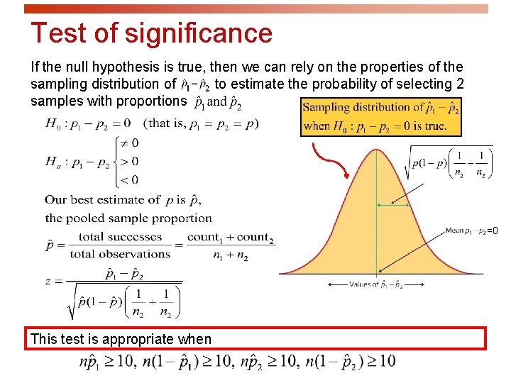
Test of significance If the null hypothesis is true, then we can rely on the properties of the sampling distribution of to estimate the probability of selecting 2 samples with proportions =0 This test is appropriate when

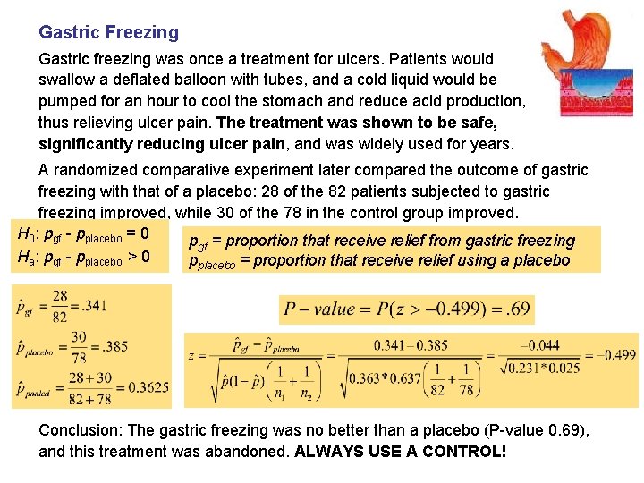
Gastric Freezing Gastric freezing was once a treatment for ulcers. Patients would swallow a deflated balloon with tubes, and a cold liquid would be pumped for an hour to cool the stomach and reduce acid production, thus relieving ulcer pain. The treatment was shown to be safe, significantly reducing ulcer pain, and was widely used for years. A randomized comparative experiment later compared the outcome of gastric freezing with that of a placebo: 28 of the 82 patients subjected to gastric freezing improved, while 30 of the 78 in the control group improved. H 0: pgf - pplacebo = 0 pgf = proportion that receive relief from gastric freezing Ha: pgf - pplacebo > 0 pplacebo = proportion that receive relief using a placebo Conclusion: The gastric freezing was no better than a placebo (P-value 0. 69), and this treatment was abandoned. ALWAYS USE A CONTROL!

Chapter 9 (cont. ) Comparing Means: Confidence Intervals and Hypotheses Tests for the Difference between Two Population Means µ 1 - µ 2 10

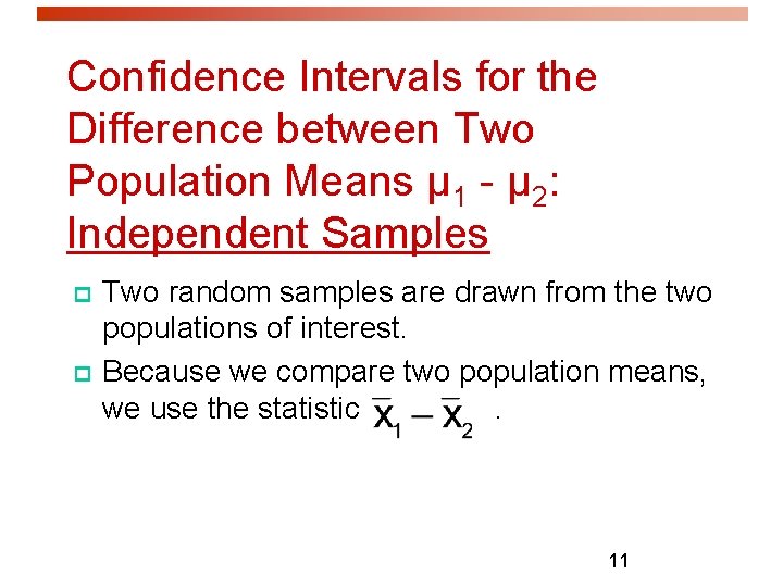
Confidence Intervals for the Difference between Two Population Means µ 1 - µ 2: Independent Samples p p Two random samples are drawn from the two populations of interest. Because we compare two population means, we use the statistic. 11

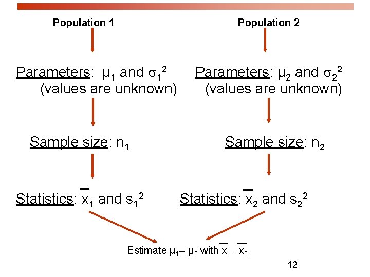
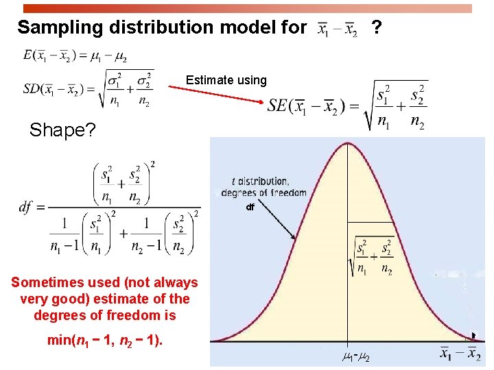
Population 1 Population 2 Parameters: µ 1 and 12 (values are unknown) Sample size: n 1 Statistics: x 1 and s 12 Parameters: µ 2 and 22 (values are unknown) Sample size: n 2 Statistics: x 2 and s 22 Estimate µ 1 µ 2 with x 1 x 2 12

Sampling distribution model for ? Estimate using Shape? df Sometimes used (not always very good) estimate of the degrees of freedom is min(n 1 − 1, n 2 − 1). m 1 -m 2

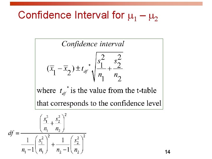
Confidence Interval for m 1 – m 2 14

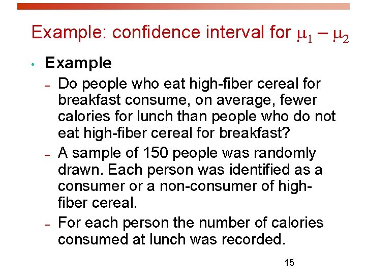
Example: confidence interval for m 1 – m 2 • Example – – – Do people who eat high-fiber cereal for breakfast consume, on average, fewer calories for lunch than people who do not eat high-fiber cereal for breakfast? A sample of 150 people was randomly drawn. Each person was identified as a consumer or a non-consumer of highfiber cereal. For each person the number of calories consumed at lunch was recorded. 15

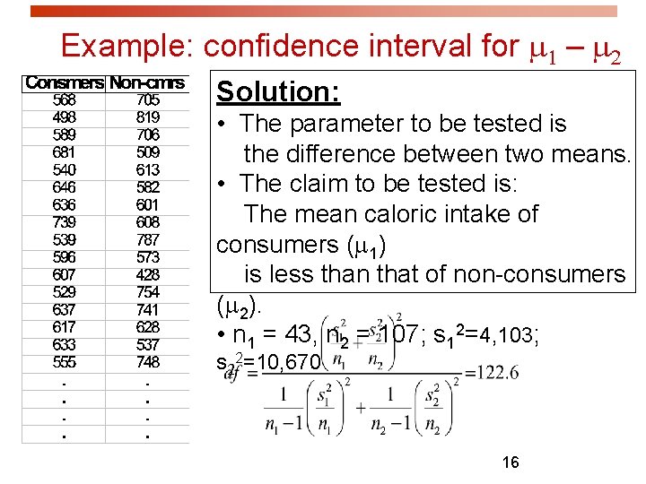
Example: confidence interval for m 1 – m 2 Solution: • The parameter to be tested is the difference between two means. • The claim to be tested is: The mean caloric intake of consumers (m 1) is less than that of non-consumers (m 2). • n 1 = 43, n 2 = 107; s 12=4, 103; s 22=10, 670 16

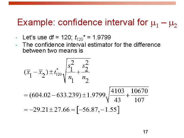
Example: confidence interval for m 1 – m 2 • • Let’s use df = 120; t 120* = 1. 9799 The confidence interval estimator for the difference between two means is 17

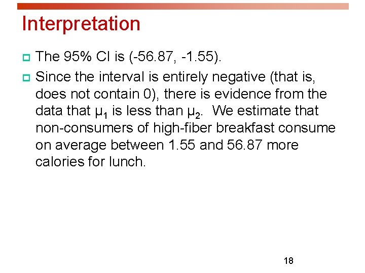
Interpretation p p The 95% CI is (-56. 87, -1. 55). Since the interval is entirely negative (that is, does not contain 0), there is evidence from the data that µ 1 is less than µ 2. We estimate that non-consumers of high-fiber breakfast consume on average between 1. 55 and 56. 87 more calories for lunch. 18

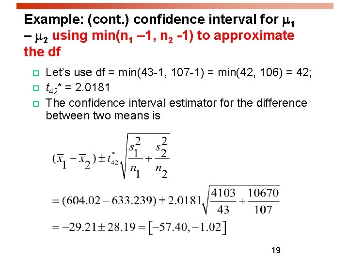
Example: (cont. ) confidence interval for 1 – 2 using min(n 1 – 1, n 2 -1) to approximate the df p p p Let’s use df = min(43 -1, 107 -1) = min(42, 106) = 42; t 42* = 2. 0181 The confidence interval estimator for the difference between two means is 19

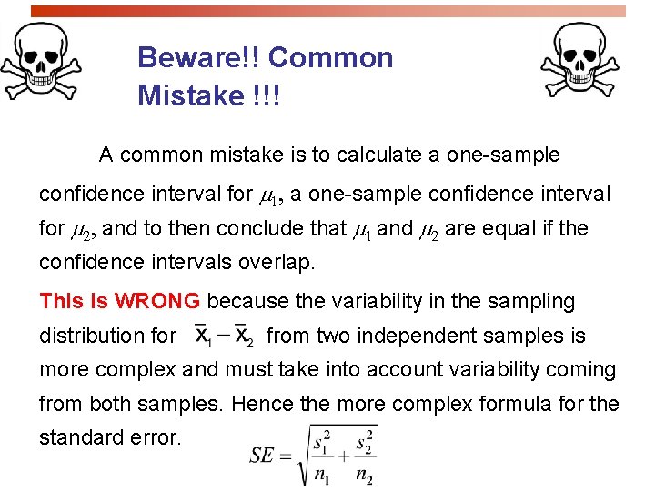
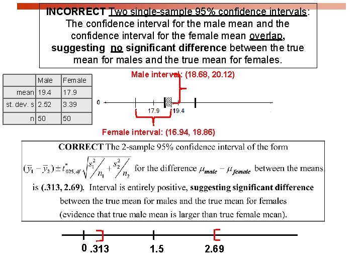
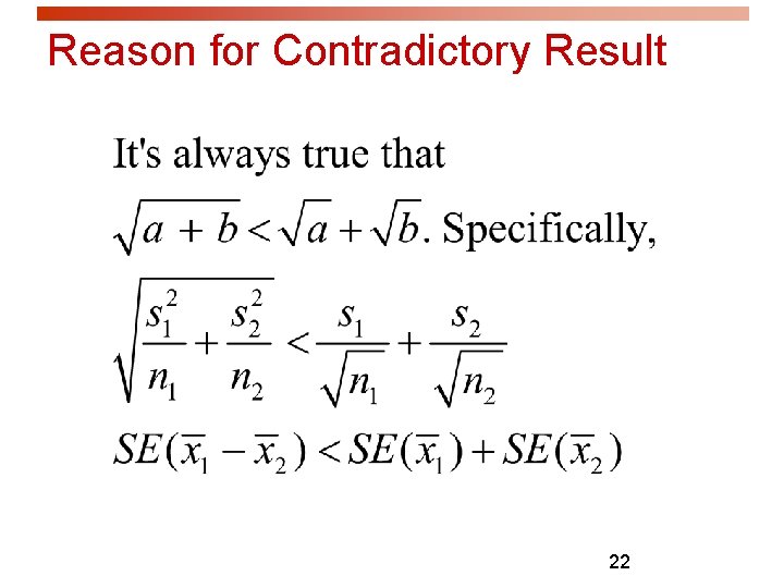
Beware!! Common Mistake !!! A common mistake is to calculate a one-sample confidence interval for m 1, a one-sample confidence interval for m 2, and to then conclude that m 1 and m 2 are equal if the confidence intervals overlap. This is WRONG because the variability in the sampling distribution for from two independent samples is more complex and must take into account variability coming from both samples. Hence the more complex formula for the standard error.

INCORRECT Two single-sample 95% confidence intervals: The confidence interval for the male mean and the confidence interval for the female mean overlap, suggesting no significant difference between the true mean for males and the true mean for females. Male mean 19. 4 17. 9 st. dev. s 2. 52 3. 39 n 50 Male interval: (18. 68, 20. 12) Female 50 Female interval: (16. 94, 18. 86) 0. 313 1. 5 2. 69

Reason for Contradictory Result 22

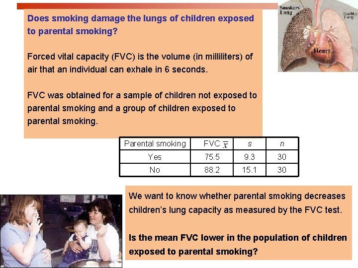
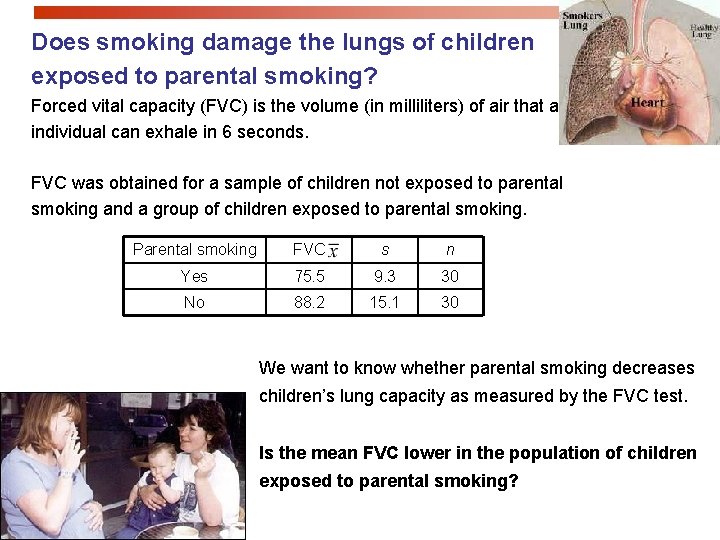
Does smoking damage the lungs of children exposed to parental smoking? Forced vital capacity (FVC) is the volume (in milliliters) of air that an individual can exhale in 6 seconds. FVC was obtained for a sample of children not exposed to parental smoking and a group of children exposed to parental smoking. Parental smoking FVC s n Yes 75. 5 9. 3 30 No 88. 2 15. 1 30 We want to know whether parental smoking decreases children’s lung capacity as measured by the FVC test. Is the mean FVC lower in the population of children exposed to parental smoking?

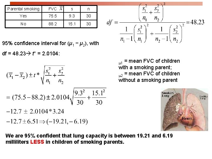
Parental smoking FVC s n Yes 75. 5 9. 3 30 No 88. 2 15. 1 30 95% confidence interval for (µ 1 − µ 2), with df = 48. 23 t* = 2. 0104: = mean FVC of children with a smoking parent; m 2 = mean FVC of children without a smoking parent m 1 We are 95% confident that lung capacity is between 19. 21 and 6. 19 milliliters LESS in children of smoking parents.

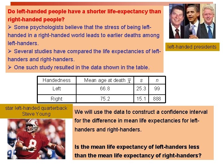
Do left-handed people have a shorter life-expectancy than right-handed people? Ø Some psychologists believe that the stress of being lefthanded in a right-handed world leads to earlier deaths among left-handers. Ø Several studies have compared the life expectancies of lefthanders and right-handers. Ø One such study resulted in the data shown in the table. Handedness Mean age at death s n Left 66. 8 25. 3 99 Right 75. 2 15. 1 888 star left-handed quarterback Steve Young left-handed presidents We will use the data to construct a confidence interval for the difference in mean life expectancies for lefthanders and right-handers. Is the mean life expectancy of left-handers less than the mean life expectancy of right-handers?

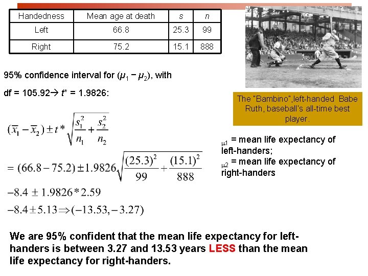
Handedness Mean age at death s n Left 66. 8 25. 3 99 Right 75. 2 15. 1 888 95% confidence interval for (µ 1 − µ 2), with df = 105. 92 t* = 1. 9826: The “Bambino”, left-handed Babe Ruth, baseball’s all-time best player. = mean life expectancy of left-handers; m 2 = mean life expectancy of right-handers m 1 We are 95% confident that the mean life expectancy for lefthanders is between 3. 27 and 13. 53 years LESS than the mean life expectancy for right-handers.

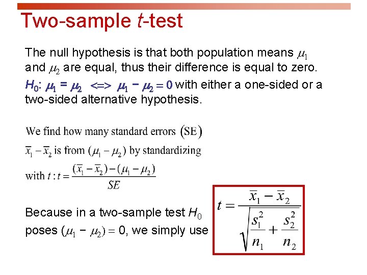
Two-sample t-test The null hypothesis is that both population means m 1 and m 2 are equal, thus their difference is equal to zero. H 0: m 1 = m 2 <=> m 1 − m 2 = 0 with either a one-sided or a two-sided alternative hypothesis. Because in a two-sample test H 0 poses (m 1 − m 2) = 0, we simply use

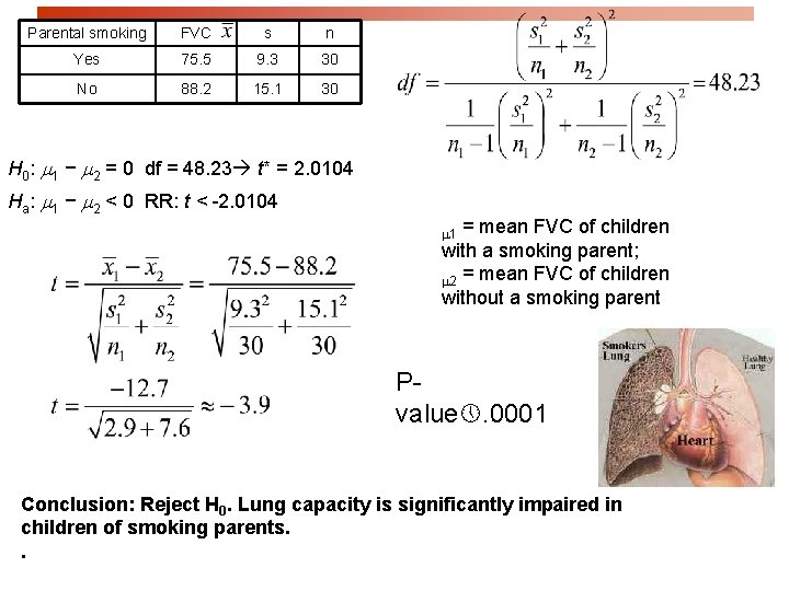
Does smoking damage the lungs of children exposed to parental smoking? Forced vital capacity (FVC) is the volume (in milliliters) of air that an individual can exhale in 6 seconds. FVC was obtained for a sample of children not exposed to parental smoking and a group of children exposed to parental smoking. Parental smoking FVC s n Yes 75. 5 9. 3 30 No 88. 2 15. 1 30 We want to know whether parental smoking decreases children’s lung capacity as measured by the FVC test. Is the mean FVC lower in the population of children exposed to parental smoking?

Parental smoking FVC s n Yes 75. 5 9. 3 30 No 88. 2 15. 1 30 H 0: m 1 − m 2 = 0 df = 48. 23 t* = 2. 0104 Ha: m 1 − m 2 < 0 RR: t < -2. 0104 = mean FVC of children with a smoking parent; m 2 = mean FVC of children without a smoking parent m 1 Pvalue. 0001 Conclusion: Reject H 0. Lung capacity is significantly impaired in children of smoking parents. .

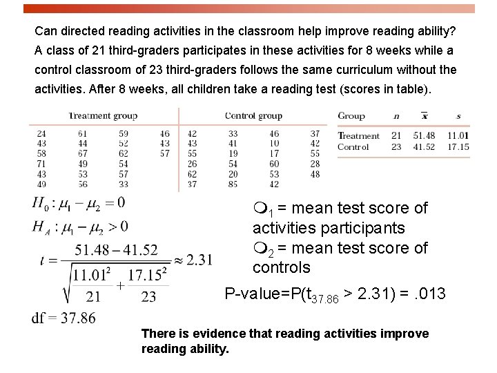
Can directed reading activities in the classroom help improve reading ability? A class of 21 third-graders participates in these activities for 8 weeks while a control classroom of 23 third-graders follows the same curriculum without the activities. After 8 weeks, all children take a reading test (scores in table). 1 = mean test score of activities participants 2 = mean test score of controls P-value=P(t 37. 86 > 2. 31) =. 013 There is evidence that reading activities improve reading ability.

Robustness The two-sample t procedures are more robust than the onesample t procedures. They are the most robust when both sample sizes are equal and both sample distributions are similar. But even when we deviate from this, two-sample tests tend to remain quite robust. When planning a two-sample study, choose equal sample sizes if you can. As a guideline, a combined sample size (n 1 + n 2) of 40 or more will allow you to work even with the most skewed distributions.

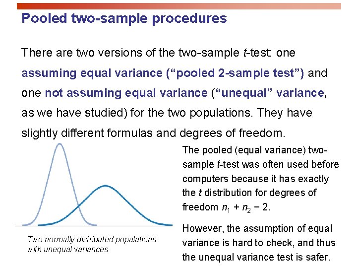
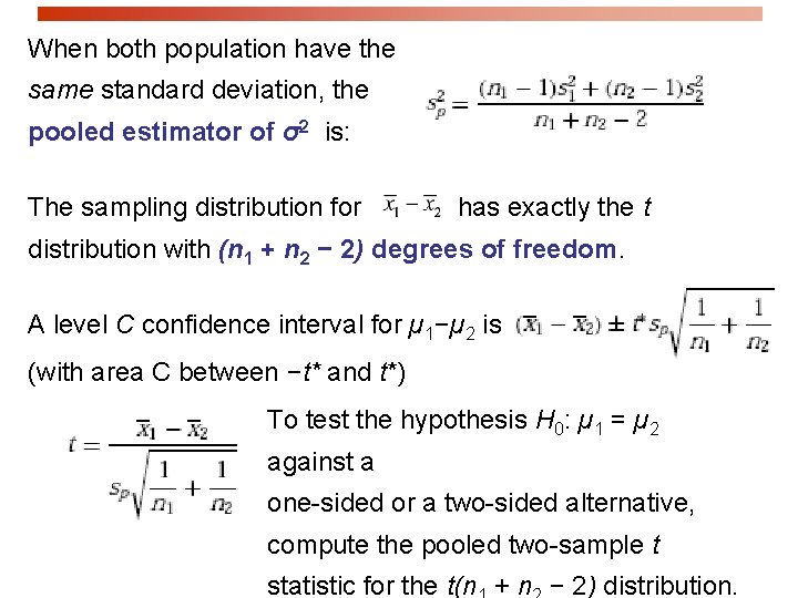
Pooled two-sample procedures There are two versions of the two-sample t-test: one assuming equal variance (“pooled 2 -sample test”) and one not assuming equal variance (“unequal” variance, as we have studied) for the two populations. They have slightly different formulas and degrees of freedom. The pooled (equal variance) twosample t-test was often used before computers because it has exactly the t distribution for degrees of freedom n 1 + n 2 − 2. Two normally distributed populations with unequal variances However, the assumption of equal variance is hard to check, and thus the unequal variance test is safer.

When both population have the same standard deviation, the pooled estimator of σ2 is: The sampling distribution for has exactly the t distribution with (n 1 + n 2 − 2) degrees of freedom. A level C confidence interval for µ 1−µ 2 is (with area C between −t* and t*) To test the hypothesis H 0: µ 1 = µ 2 against a one-sided or a two-sided alternative, compute the pooled two-sample t statistic for the t(n + n − 2) distribution.

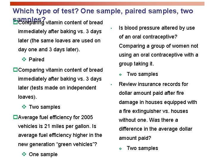
Which type of test? One sample, paired samples, two samples? p Comparing vitamin content of bread immediately after baking vs. 3 days • of an oral contraceptive? later (the same loaves are used on Comparing a group of women not day one and 3 days later). using an oral contraceptive with a v Paired group taking it. p. Comparing vitamin content of bread v immediately after baking vs. 3 days later (tests made on independent loaves). v Two samples p. Average fuel efficiency for 2005 vehicles is 21 miles per gallon. Is average fuel efficiency higher in the new generation “green vehicles”? v One sample Is blood pressure altered by use • Two samples Review insurance records for dollar amount paid after fire damage in houses equipped with a fire extinguisher vs. houses without one. Was there a difference in the average dollar amount paid? v Two samples