Significance Testing for Comparing Two Means Comparing Two

Significance Testing for Comparing Two Means

Comparing Two Means After this section, you should be able to… ü DETERMINE whether the conditions for performing inference are met ü USE two-sample t procedures to compare two means based on summary statistics or raw data ü INTERPRET computer output for two-sample t procedures ü PERFORM a significance test to compare two means ü INTERPRET the results of inference procedures ü ANALYZE the distribution of differences in a paired data set using graphs and summary statistics ü DETERMINE when it is appropriate to use paired t procedures vs. two sample t procedures.

Significance Tests for µ 1 – µ 2 • An observed difference between two sample means can reflect an actual difference in the parameters, or it may just be due to chance variation in random sampling or random assignment. • Significance tests help us decide which explanation makes more sense. • The null hypothesis has the general form: H 0: µ 1 = µ 2 • The alternative hypothesis says what kind of difference we expect: H a: µ 1 > µ 2 OR H a: µ 1 < µ 2 OR H a: µ 1 ≠ µ 2

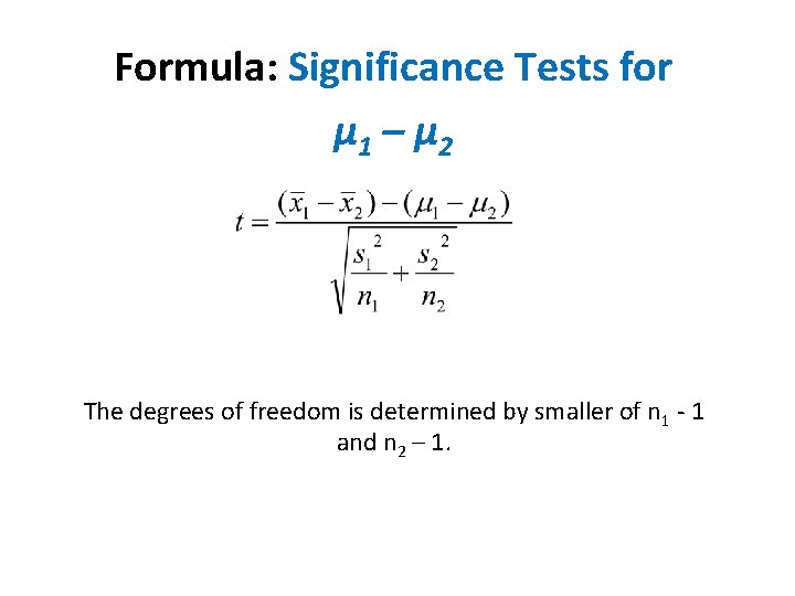
Formula: Significance Tests for µ 1 – µ 2 The degrees of freedom is determined by smaller of n 1 - 1 and n 2 – 1.

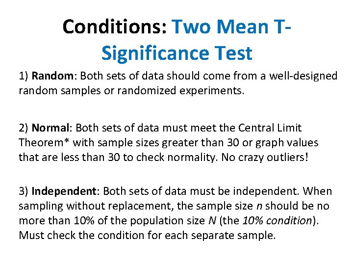
Conditions: Two Mean TSignificance Test 1) Random: Both sets of data should come from a well-designed random samples or randomized experiments. 2) Normal: Both sets of data must meet the Central Limit Theorem* with sample sizes greater than 30 or graph values that are less than 30 to check normality. No crazy outliers! 3) Independent: Both sets of data must be independent. When sampling without replacement, the sample size n should be no more than 10% of the population size N (the 10% condition). Must check the condition for each separate sample.

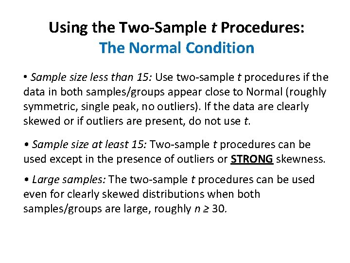
Using the Two-Sample t Procedures: The Normal Condition • Sample size less than 15: Use two-sample t procedures if the data in both samples/groups appear close to Normal (roughly symmetric, single peak, no outliers). If the data are clearly skewed or if outliers are present, do not use t. • Sample size at least 15: Two-sample t procedures can be used except in the presence of outliers or STRONG skewness. • Large samples: The two-sample t procedures can be used even for clearly skewed distributions when both samples/groups are large, roughly n ≥ 30.

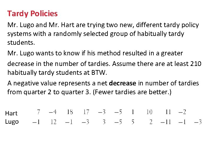
Tardy Policies Mr. Lugo and Mr. Hart are trying two new, different tardy policy systems with a randomly selected group of habitually tardy students. Mr. Lugo wants to know if his method resulted in a greater decrease in the number of tardies. Assume there at least 210 habitually tardy students at BTW. A negative value represents a net decrease in number of tardies from quarter 2 to quarter 3. (Fewer tardies are better. ) Hart Lugo

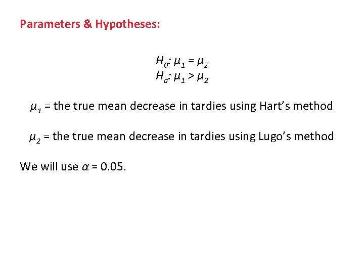
Parameters & Hypotheses: H 0 : µ 1 = µ 2 Ha : µ 1 > µ 2 µ 1 = the true mean decrease in tardies using Hart’s method µ 2 = the true mean decrease in tardies using Lugo’s method We will use α = 0. 05.

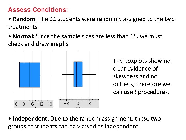
Assess Conditions: • Random: The 21 students were randomly assigned to the two treatments. • Normal: Since the sample sizes are less than 15, we must check and draw graphs. The boxplots show no clear evidence of skewness and no outliers, therefore we can use t procedures. • Independent: Due to the random assignment, these two groups of students can be viewed as independent.

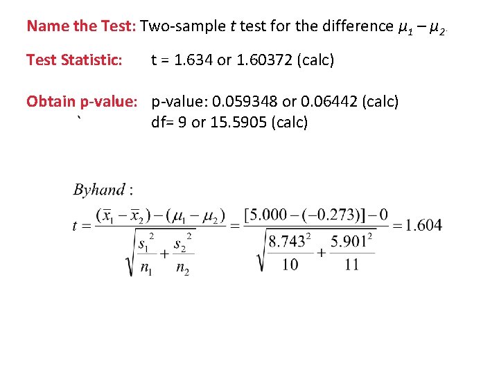
Name the Test: Two-sample t test for the difference µ 1 – µ 2. Test Statistic: t = 1. 634 or 1. 60372 (calc) Obtain p-value: 0. 059348 or 0. 06442 (calc) ` df= 9 or 15. 5905 (calc)

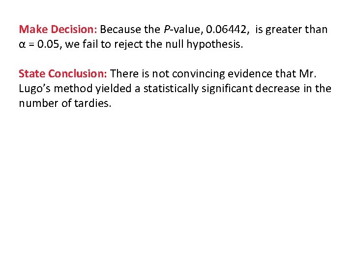
Make Decision: Because the P-value, 0. 06442, is greater than α = 0. 05, we fail to reject the null hypothesis. State Conclusion: There is not convincing evidence that Mr. Lugo’s method yielded a statistically significant decrease in the number of tardies.

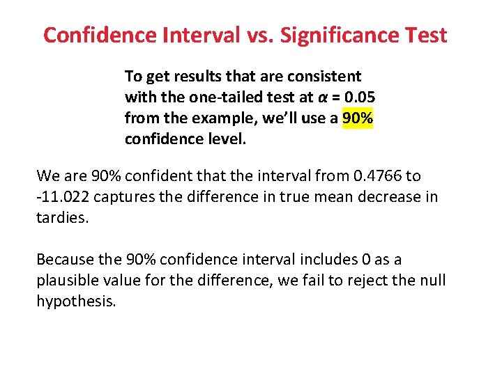
Confidence Interval vs. Significance Test To get results that are consistent with the one-tailed test at α = 0. 05 from the example, we’ll use a 90% confidence level. We are 90% confident that the interval from 0. 4766 to -11. 022 captures the difference in true mean decrease in tardies. Because the 90% confidence interval includes 0 as a plausible value for the difference, we fail to reject the null hypothesis.

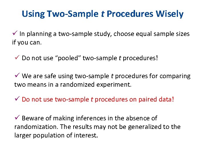
Using Two-Sample t Procedures Wisely ü In planning a two-sample study, choose equal sample sizes if you can. ü Do not use “pooled” two-sample t procedures! ü We are safe using two-sample t procedures for comparing two means in a randomized experiment. ü Do not use two-sample t procedures on paired data! ü Beware of making inferences in the absence of randomization. The results may not be generalized to the larger population of interest.

Comparing Two Means: Paired Data

Section 10. 3 Comparing Two Means: Paired Data After this section, you should be able to…

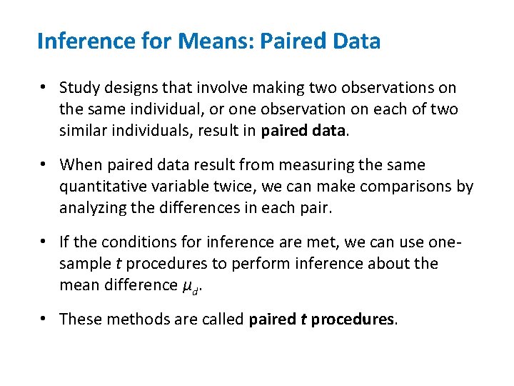
Inference for Means: Paired Data • Study designs that involve making two observations on the same individual, or one observation on each of two similar individuals, result in paired data. • When paired data result from measuring the same quantitative variable twice, we can make comparisons by analyzing the differences in each pair. • If the conditions for inference are met, we can use onesample t procedures to perform inference about the mean difference µd. • These methods are called paired t procedures.

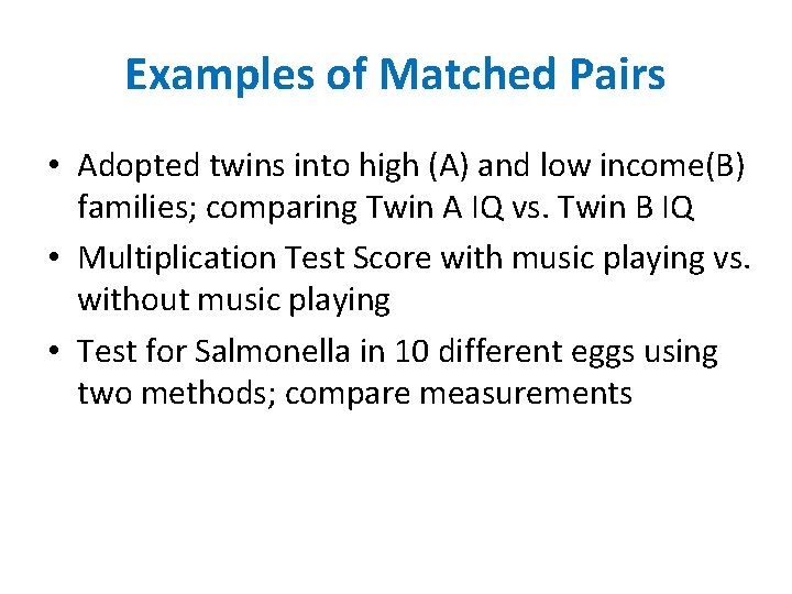
Examples of Matched Pairs • Adopted twins into high (A) and low income(B) families; comparing Twin A IQ vs. Twin B IQ • Multiplication Test Score with music playing vs. without music playing • Test for Salmonella in 10 different eggs using two methods; compare measurements

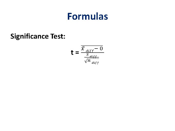
Formulas •

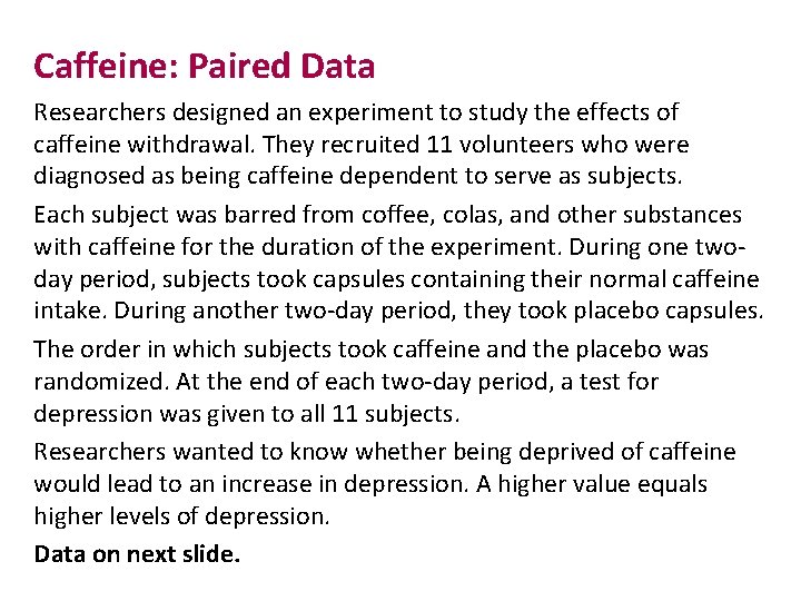
Caffeine: Paired Data Researchers designed an experiment to study the effects of caffeine withdrawal. They recruited 11 volunteers who were diagnosed as being caffeine dependent to serve as subjects. Each subject was barred from coffee, colas, and other substances with caffeine for the duration of the experiment. During one twoday period, subjects took capsules containing their normal caffeine intake. During another two-day period, they took placebo capsules. The order in which subjects took caffeine and the placebo was randomized. At the end of each two-day period, a test for depression was given to all 11 subjects. Researchers wanted to know whether being deprived of caffeine would lead to an increase in depression. A higher value equals higher levels of depression. Data on next slide.

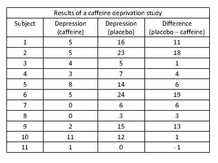
Results of a caffeine deprivation study Subject Depression (caffeine) Depression (placebo) Difference (placebo – caffeine) 1 5 16 11 2 5 23 18 3 4 5 1 4 3 7 4 5 8 14 6 6 5 24 19 7 0 6 6 8 0 3 3 9 2 15 13 10 11 12 1 11 1 0 -1

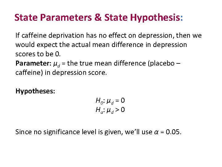
State Parameters & State Hypothesis: If caffeine deprivation has no effect on depression, then we would expect the actual mean difference in depression scores to be 0. Parameter: µd = the true mean difference (placebo – caffeine) in depression score. Hypotheses: H 0 : µ d = 0 Ha : µ d > 0 Since no significance level is given, we’ll use α = 0. 05.

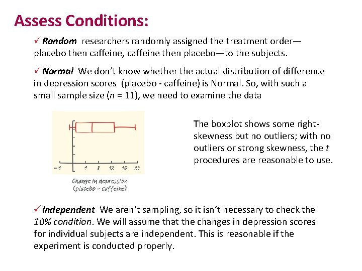
Assess Conditions: üRandom researchers randomly assigned the treatment order— placebo then caffeine, caffeine then placebo—to the subjects. üNormal We don’t know whether the actual distribution of difference in depression scores (placebo - caffeine) is Normal. So, with such a small sample size (n = 11), we need to examine the data The boxplot shows some rightskewness but no outliers; with no outliers or strong skewness, the t procedures are reasonable to use. üIndependent We aren’t sampling, so it isn’t necessary to check the 10% condition. We will assume that the changes in depression scores for individual subjects are independent. This is reasonable if the experiment is conducted properly.

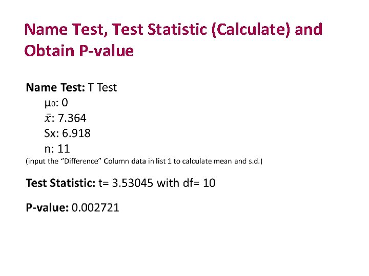
Name Test, Test Statistic (Calculate) and Obtain P-value

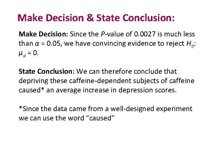
Make Decision & State Conclusion: Make Decision: Since the P-value of 0. 0027 is much less than α = 0. 05, we have convincing evidence to reject H 0: µd = 0. State Conclusion: We can therefore conclude that depriving these caffeine-dependent subjects of caffeine caused* an average increase in depression scores. *Since the data came from a well-designed experiment we can use the word “caused”