Comparing Populations Proportions and means Comparing proportions Situation

Comparing Populations Proportions and means

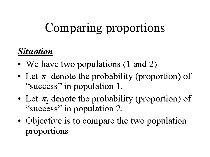
Comparing proportions Situation • We have two populations (1 and 2) • Let p 1 denote the probability (proportion) of “success” in population 1. • Let p 2 denote the probability (proportion) of “success” in population 2. • Objective is to compare the two population proportions

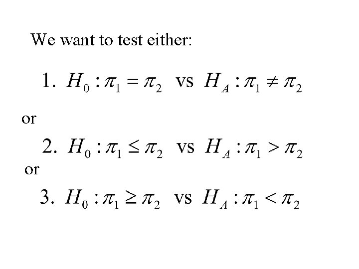
We want to test either: or or

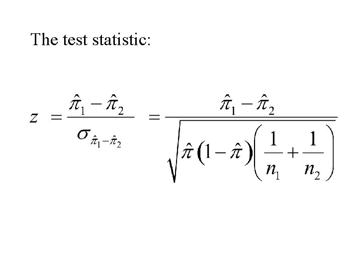
The test statistic:

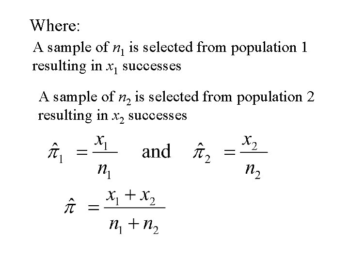
Where: A sample of n 1 is selected from population 1 resulting in x 1 successes A sample of n 2 is selected from population 2 resulting in x 2 successes

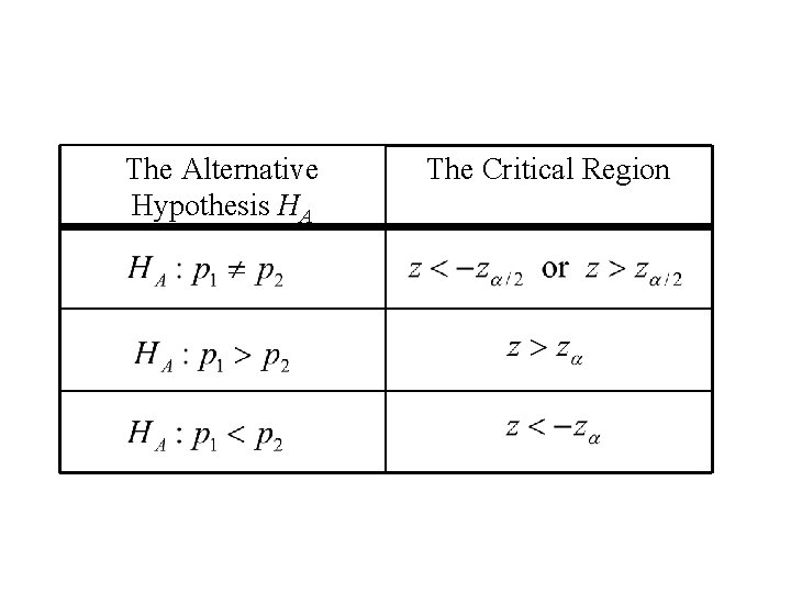
The Alternative Hypothesis HA The Critical Region

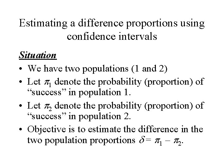
Estimating a difference proportions using confidence intervals Situation • We have two populations (1 and 2) • Let p 1 denote the probability (proportion) of “success” in population 1. • Let p 2 denote the probability (proportion) of “success” in population 2. • Objective is to estimate the difference in the two population proportions d = p 1 – p 2.

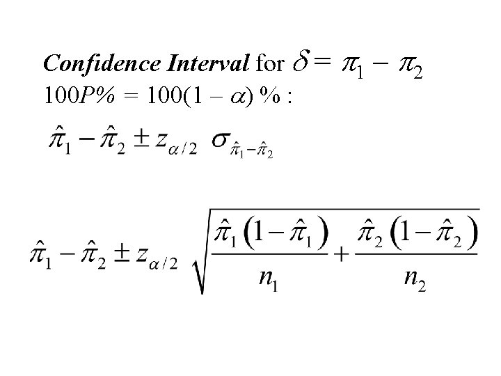
Confidence Interval for d 100 P% = 100(1 – a) % : = p 1 – p 2

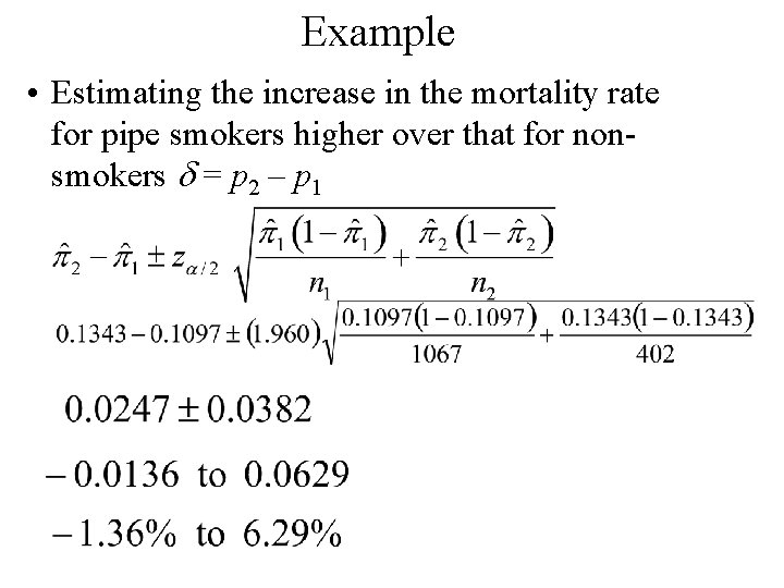
Example • Estimating the increase in the mortality rate for pipe smokers higher over that for nonsmokers d = p 2 – p 1

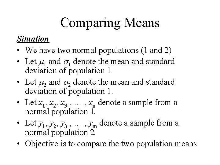
Comparing Means Situation • We have two normal populations (1 and 2) • Let m 1 and s 1 denote the mean and standard deviation of population 1. • Let m 2 and s 2 denote the mean and standard deviation of population 1. • Let x 1, x 2, x 3 , … , xn denote a sample from a normal population 1. • Let y 1, y 2, y 3 , … , ym denote a sample from a normal population 2. • Objective is to compare the two population means

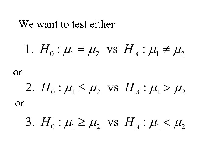
We want to test either: or or

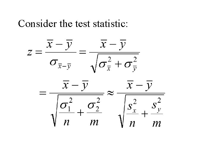
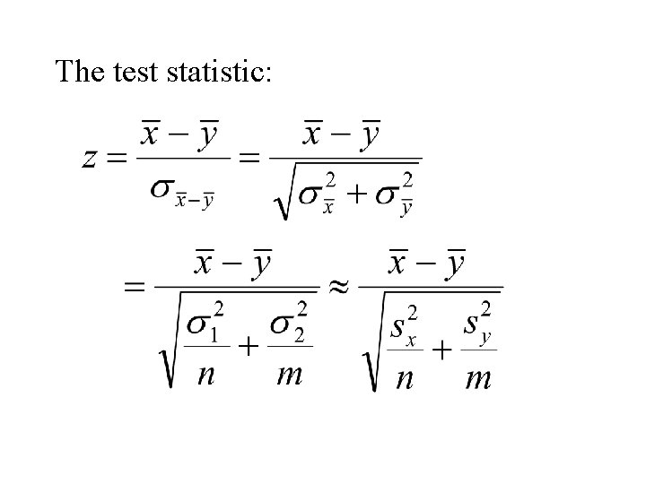
Consider the test statistic:

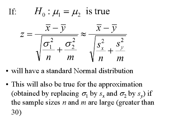
If: • will have a standard Normal distribution • This will also be true for the approximation (obtained by replacing s 1 by sx and s 2 by sy) if the sample sizes n and m are large (greater than 30)

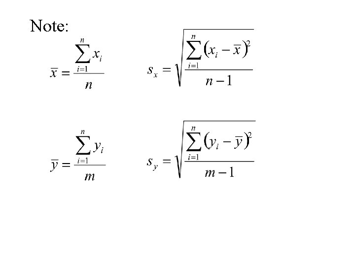
Note:

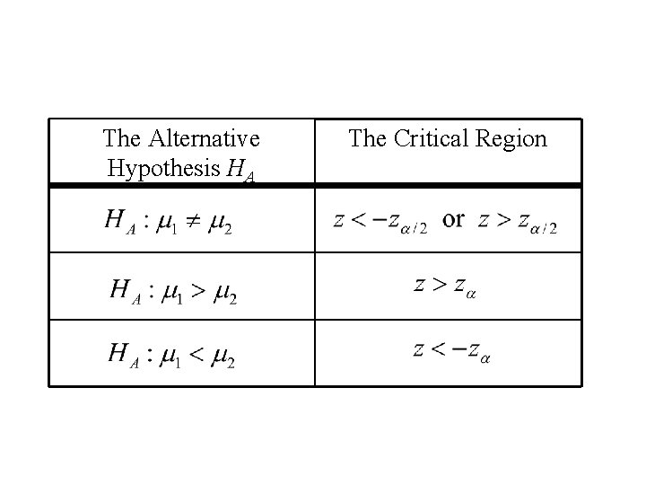
The Alternative Hypothesis HA The Critical Region

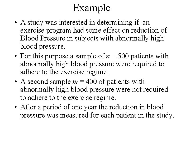
Example • A study was interested in determining if an exercise program had some effect on reduction of Blood Pressure in subjects with abnormally high blood pressure. • For this purpose a sample of n = 500 patients with abnormally high blood pressure were required to adhere to the exercise regime. • A second sample m = 400 of patients with abnormally high blood pressure were not required to adhere to the exercise regime. • After a period of one year the reduction in blood pressure was measured for each patient in the study.

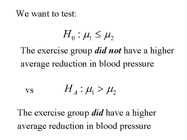
We want to test: The exercise group did not have a higher average reduction in blood pressure vs The exercise group did have a higher average reduction in blood pressure

The test statistic:

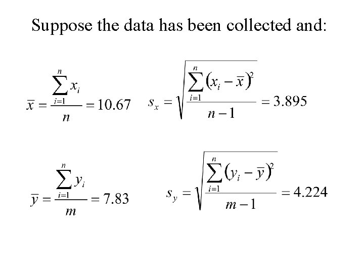
Suppose the data has been collected and:

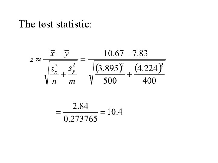
The test statistic:

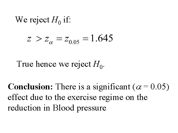
We reject H 0 if: True hence we reject H 0. Conclusion: There is a significant (a = 0. 05) effect due to the exercise regime on the reduction in Blood pressure

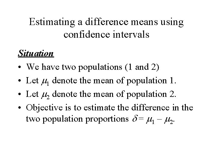
Estimating a difference means using confidence intervals Situation • We have two populations (1 and 2) • Let m 1 denote the mean of population 1. • Let m 2 denote the mean of population 2. • Objective is to estimate the difference in the two population proportions d = m 1 – m 2.

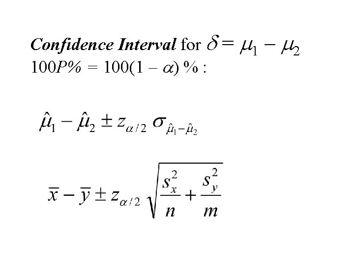
Confidence Interval for d 100 P% = 100(1 – a) % : = m 1 – m 2

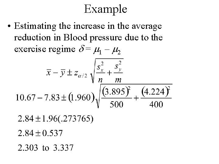
Example • Estimating the increase in the average reduction in Blood pressure due to the exercise regime d = m 1 – m 2

Sample size determination When comparing two or more populations

Estimating a difference proportions using confidence intervals Situation • We have two populations (1 and 2) • Let p 1 denote the probability (proportion) of “success” in population 1. • Let p 2 denote the probability (proportion) of “success” in population 2. • Objective is to estimate the difference in the two population proportions d = p 1 – p 2.

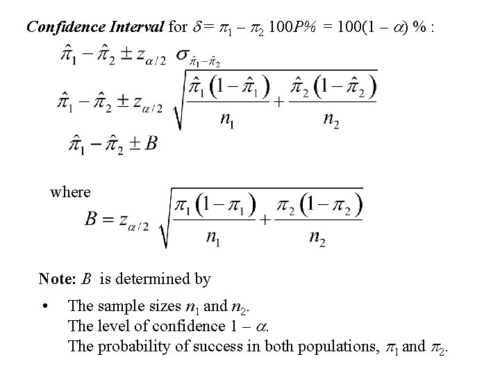
Confidence Interval for d = p 1 – p 2 100 P% = 100(1 – a) % : where Note: B is determined by • The sample sizes n 1 and n 2. The level of confidence 1 – a. The probability of success in both populations, p 1 and p 2.

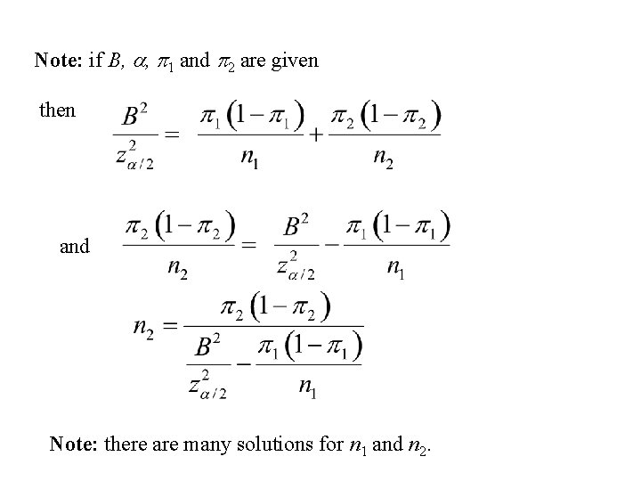
Note: if B, a, p 1 and p 2 are given then and Note: there are many solutions for n 1 and n 2.

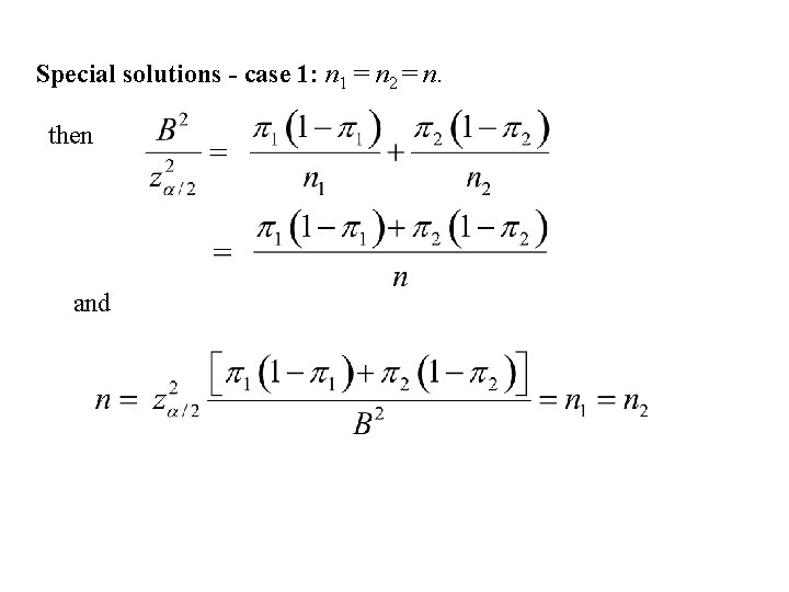
Special solutions - case 1: n 1 = n 2 = n. then and

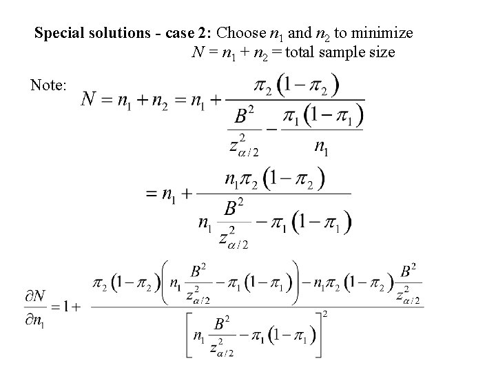
Special solutions - case 2: Choose n 1 and n 2 to minimize N = n 1 + n 2 = total sample size Note:

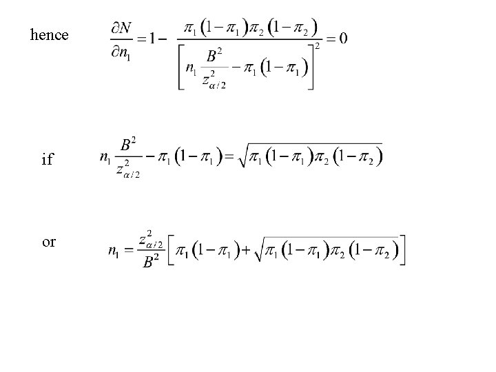
hence if or

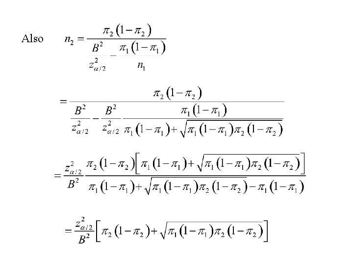
Also

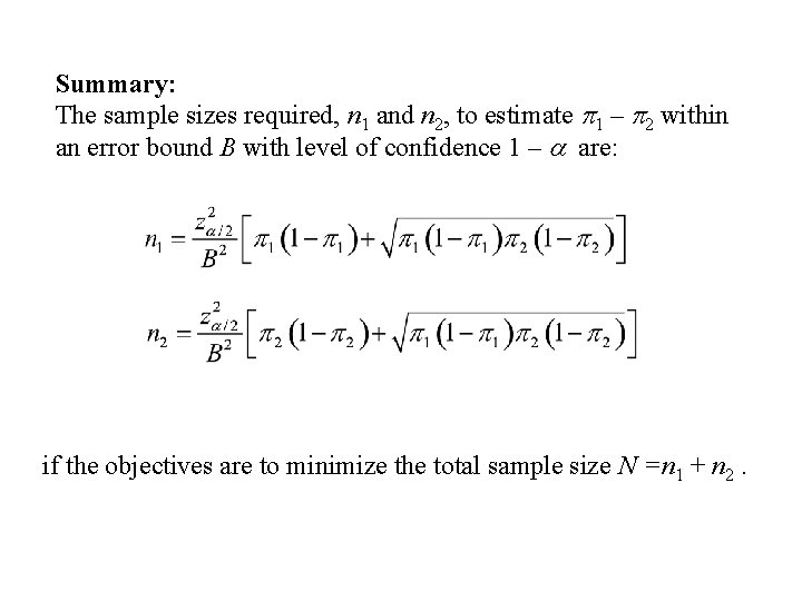
Summary: The sample sizes required, n 1 and n 2, to estimate p 1 – p 2 within an error bound B with level of confidence 1 – a are: if the objectives are to minimize the total sample size N =n 1 + n 2.

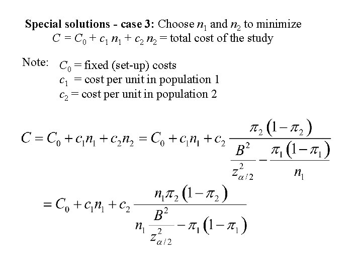
Special solutions - case 3: Choose n 1 and n 2 to minimize C = C 0 + c 1 n 1 + c 2 n 2 = total cost of the study Note: C 0 = fixed (set-up) costs c 1 = cost per unit in population 1 c 2 = cost per unit in population 2

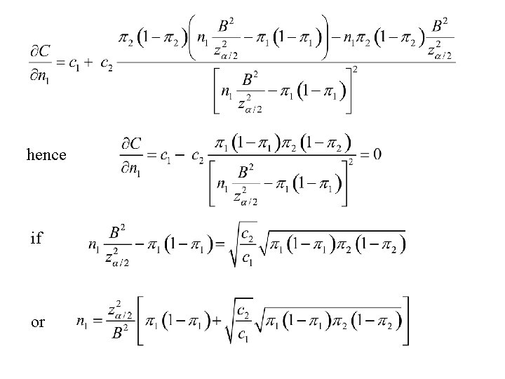
hence if or

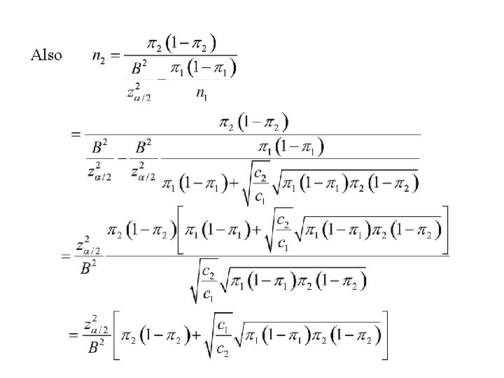
Also

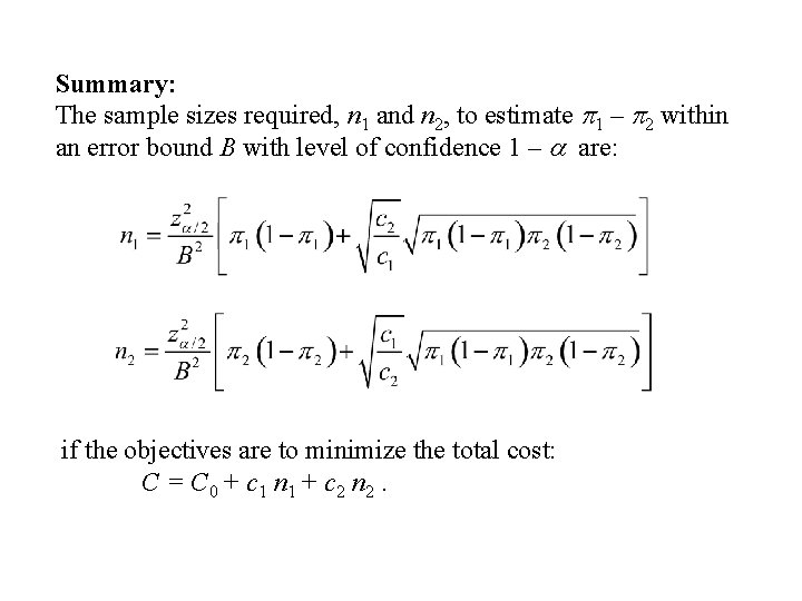
Summary: The sample sizes required, n 1 and n 2, to estimate p 1 – p 2 within an error bound B with level of confidence 1 – a are: if the objectives are to minimize the total cost: C = C 0 + c 1 n 1 + c 2 n 2.

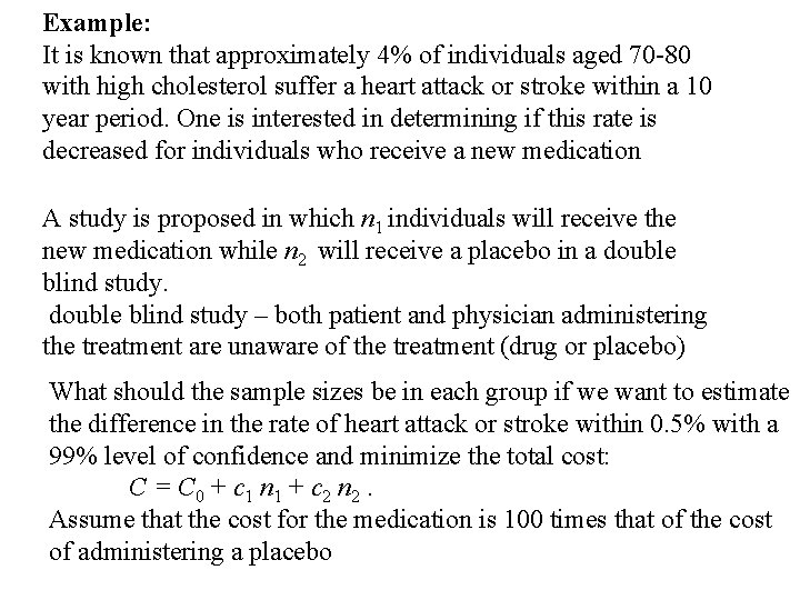
Example: It is known that approximately 4% of individuals aged 70 -80 with high cholesterol suffer a heart attack or stroke within a 10 year period. One is interested in determining if this rate is decreased for individuals who receive a new medication A study is proposed in which n 1 individuals will receive the new medication while n 2 will receive a placebo in a double blind study – both patient and physician administering the treatment are unaware of the treatment (drug or placebo) What should the sample sizes be in each group if we want to estimate the difference in the rate of heart attack or stroke within 0. 5% with a 99% level of confidence and minimize the total cost: C = C 0 + c 1 n 1 + c 2 n 2. Assume that the cost for the medication is 100 times that of the cost of administering a placebo

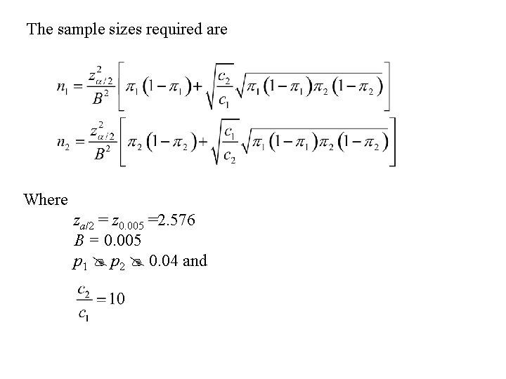
The sample sizes required are Where za/2 = z 0. 005 =2. 576 B = 0. 005 p 1 p 2 0. 04 and

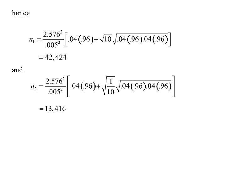
hence and

Estimating a difference means using confidence intervals Situation • We have two populations (1 and 2) • Let m 1 denote the mean of population 1. • Let m 2 denote the mean of population 2. • Objective is to estimate the difference in the two population proportions d = m 1 – m 2.

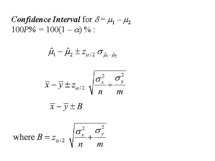
Confidence Interval for d = m 1 – m 2 100 P% = 100(1 – a) % :

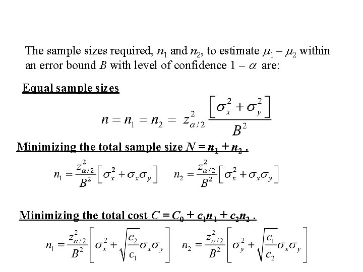
The sample sizes required, n 1 and n 2, to estimate m 1 – m 2 within an error bound B with level of confidence 1 – a are: Equal sample sizes Minimizing the total sample size N = n 1 + n 2. Minimizing the total cost C = C 0 + c 1 n 1 + c 2 n 2.

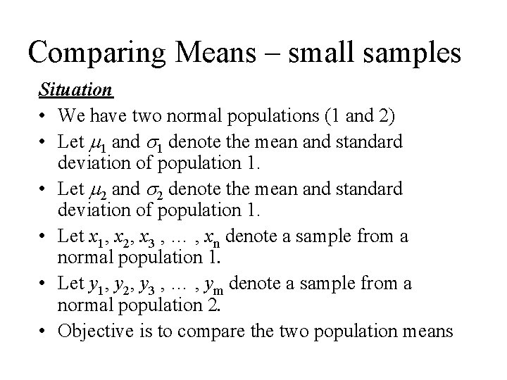
Comparing Means – small samples Situation • We have two normal populations (1 and 2) • Let m 1 and s 1 denote the mean and standard deviation of population 1. • Let m 2 and s 2 denote the mean and standard deviation of population 1. • Let x 1, x 2, x 3 , … , xn denote a sample from a normal population 1. • Let y 1, y 2, y 3 , … , ym denote a sample from a normal population 2. • Objective is to compare the two population means

We want to test either: or or

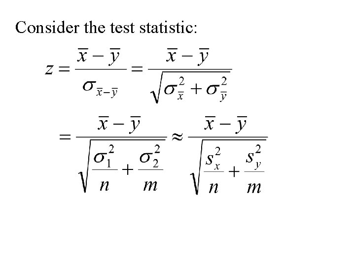
Consider the test statistic:

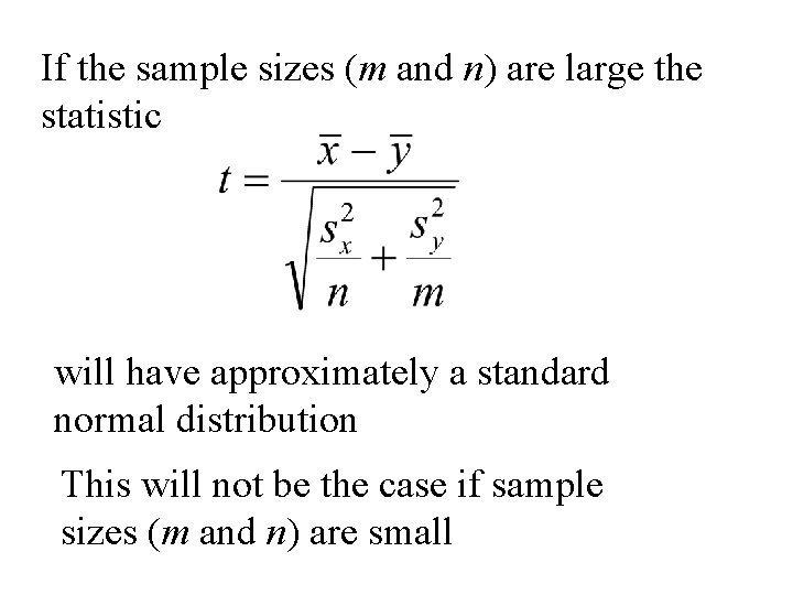
If the sample sizes (m and n) are large the statistic will have approximately a standard normal distribution This will not be the case if sample sizes (m and n) are small

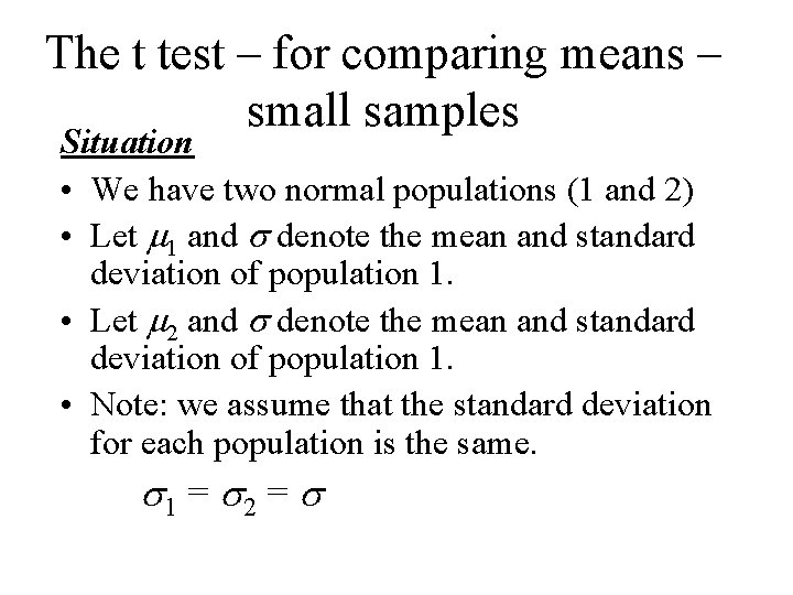
The t test – for comparing means – small samples Situation • We have two normal populations (1 and 2) • Let m 1 and s denote the mean and standard deviation of population 1. • Let m 2 and s denote the mean and standard deviation of population 1. • Note: we assume that the standard deviation for each population is the same. s 1 = s 2 = s

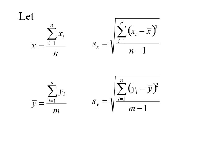
Let

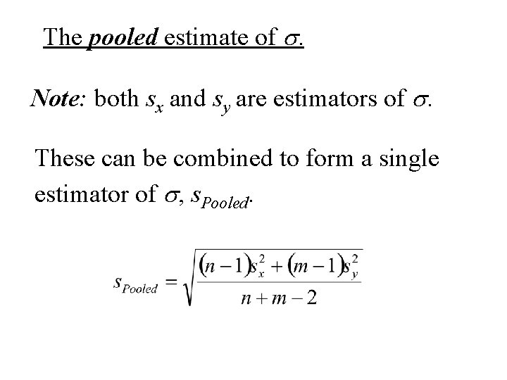
The pooled estimate of s. Note: both sx and sy are estimators of s. These can be combined to form a single estimator of s, s. Pooled.

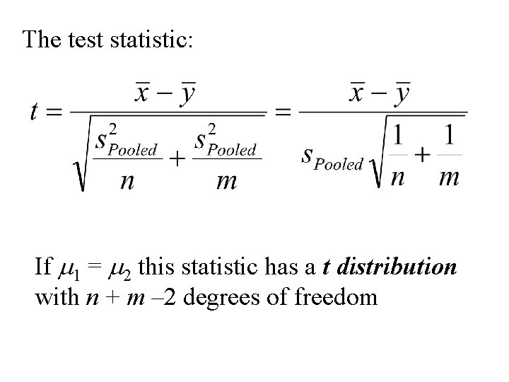
The test statistic: If m 1 = m 2 this statistic has a t distribution with n + m – 2 degrees of freedom

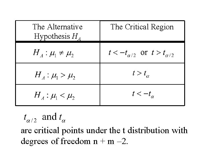
The Alternative Hypothesis HA The Critical Region are critical points under the t distribution with degrees of freedom n + m – 2.

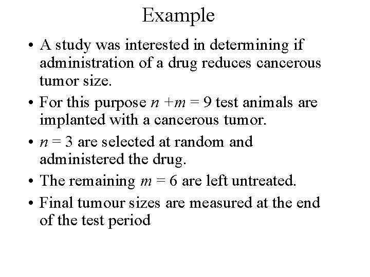
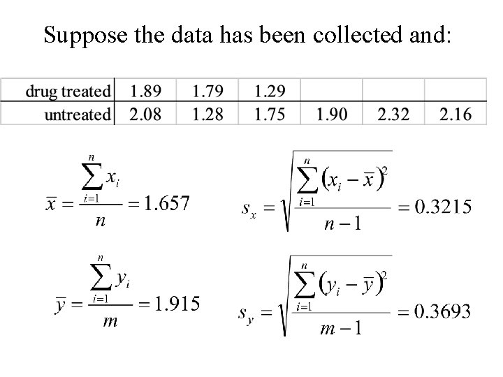
Example • A study was interested in determining if administration of a drug reduces cancerous tumor size. • For this purpose n +m = 9 test animals are implanted with a cancerous tumor. • n = 3 are selected at random and administered the drug. • The remaining m = 6 are left untreated. • Final tumour sizes are measured at the end of the test period

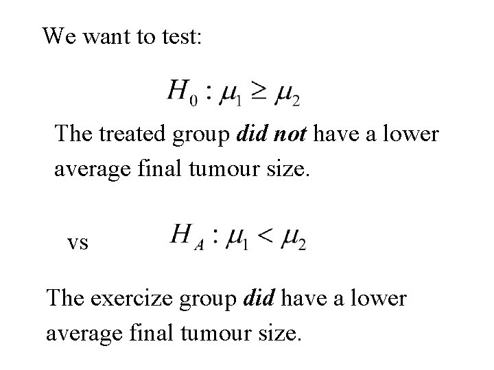
We want to test: The treated group did not have a lower average final tumour size. vs The exercize group did have a lower average final tumour size.

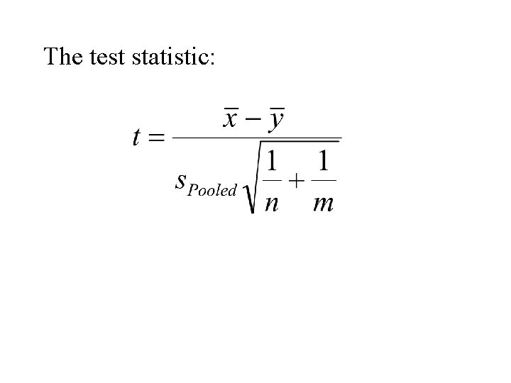
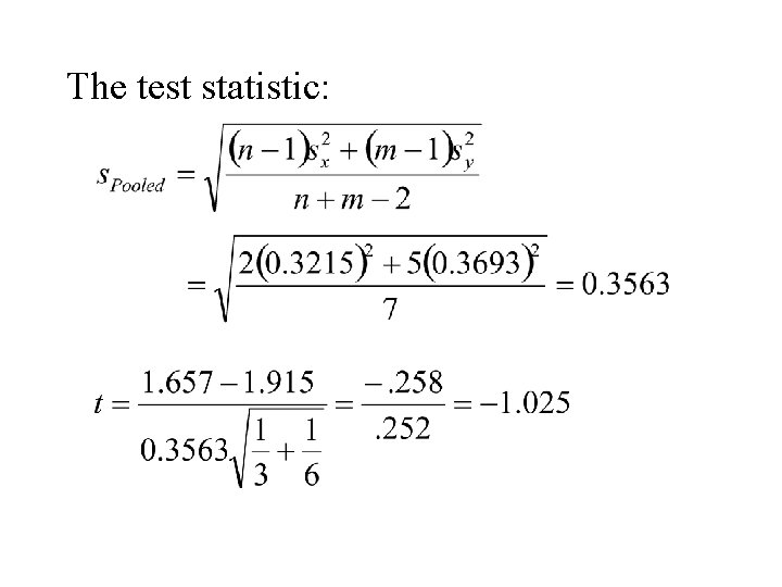
The test statistic:

Suppose the data has been collected and:

The test statistic:

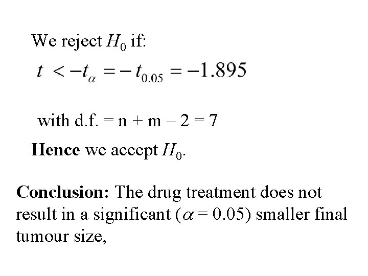
We reject H 0 if: with d. f. = n + m – 2 = 7 Hence we accept H 0. Conclusion: The drug treatment does not result in a significant (a = 0. 05) smaller final tumour size,