Chapter 10 Amortized Analysis 1 An example push

Chapter 10 Amortized Analysis 1

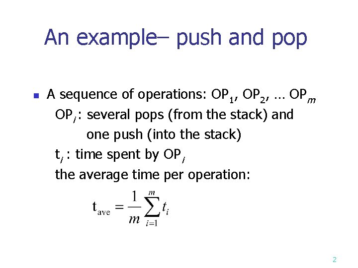
An example– push and pop A sequence of operations: OP 1, OP 2, … OPm OPi : several pops (from the stack) and one push (into the stack) ti : time spent by OPi the average time per operation: n 2

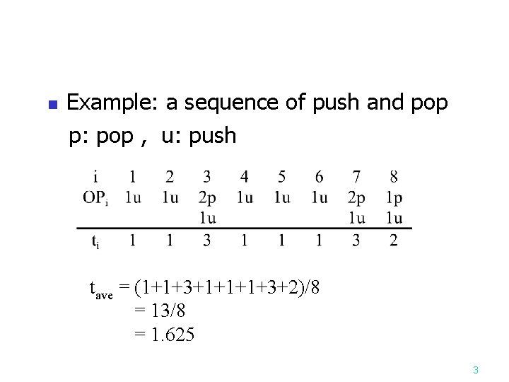
Example: a sequence of push and pop p: pop , u: push n tave = (1+1+3+1+1+1+3+2)/8 = 13/8 = 1. 625 3

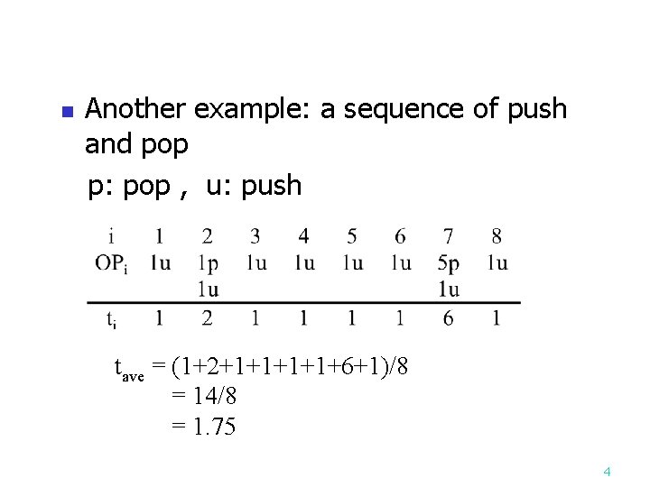
Another example: a sequence of push and pop p: pop , u: push n tave = (1+2+1+1+6+1)/8 = 14/8 = 1. 75 4

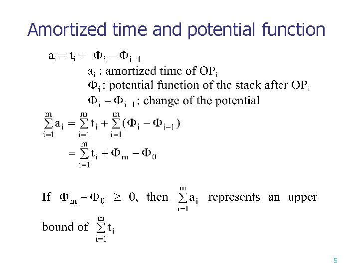
Amortized time and potential function 5

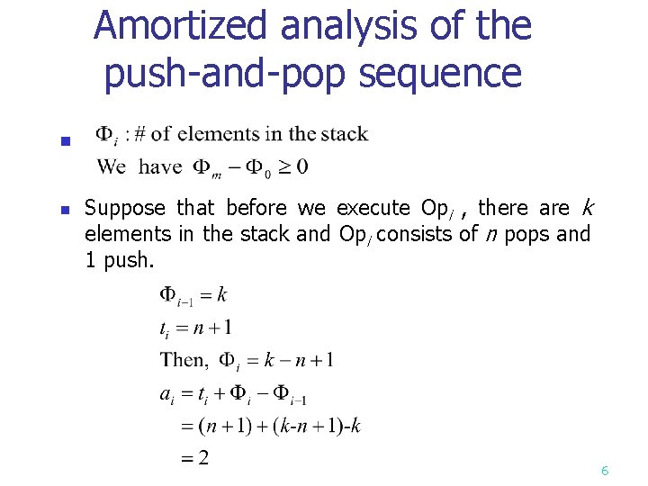
Amortized analysis of the push-and-pop sequence n n Suppose that before we execute Opi , there are k elements in the stack and Opi consists of n pops and 1 push. 6

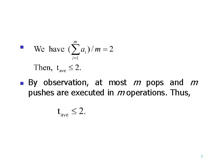
n n By observation, at most m pops and m pushes are executed in m operations. Thus, 7

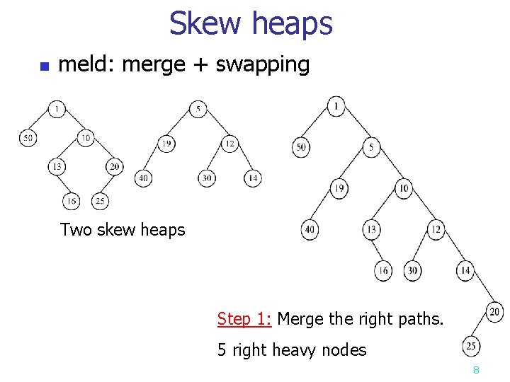
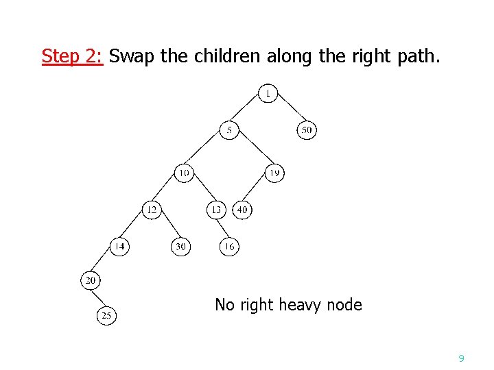
Skew heaps n meld: merge + swapping Two skew heaps Step 1: Merge the right paths. 5 right heavy nodes 8

Step 2: Swap the children along the right path. No right heavy node 9

Amortized analysis of skew heaps n n meld: merge + swapping operations on a skew heap: n n find-min(h): find the min of a skew heap h. insert(x, h): insert x into a skew heap h. delete-min(h): delete the min from a skew heap h. meld(h 1, h 2): meld two skew heaps h 1 and h 2. The first three operations can be implemented by melding. 10

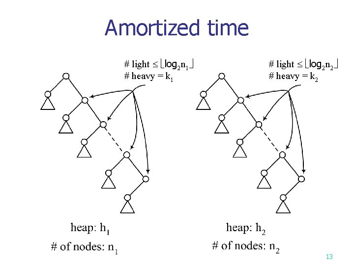
Potential function of skew heaps n n wt(x): # of descendants of node x, including x. heavy node x: wt(x) wt(p(x))/2, where p(x) is the parent node of x. light node : not a heavy node potential function i: # of right heavy nodes of the skew heap. 11

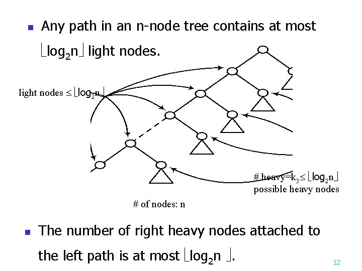
n Any path in an n-node tree contains at most log 2 n light nodes log 2 n # heavy=k 3 log 2 n possible heavy nodes # of nodes: n n The number of right heavy nodes attached to the left path is at most log 2 n . 12

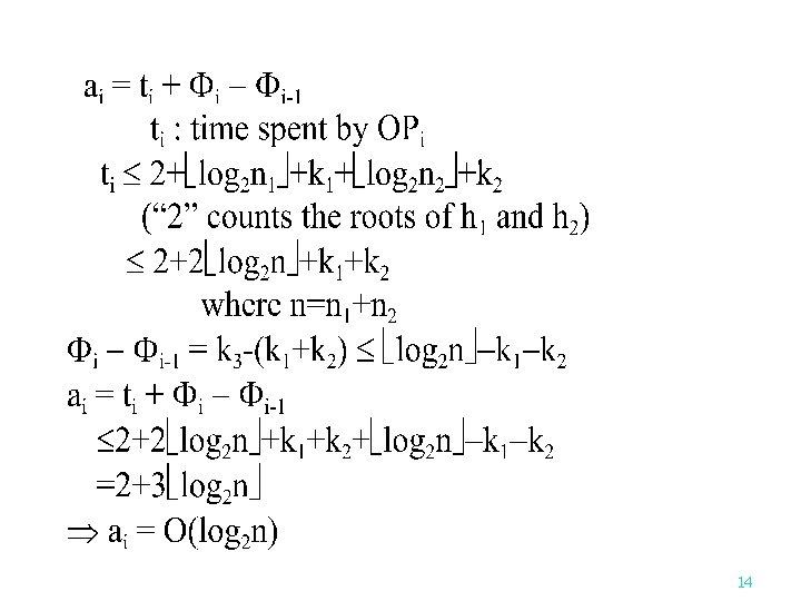
Amortized time # light log 2 n 1 # heavy = k 1 # light log 2 n 2 # heavy = k 2 13

14

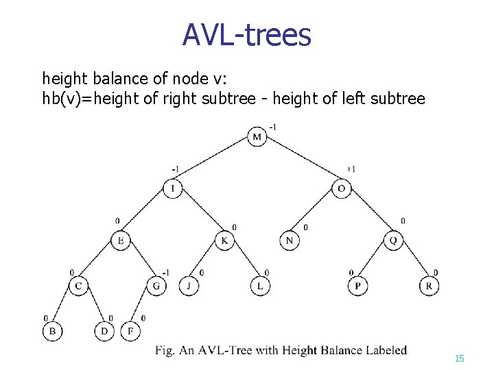
AVL-trees height balance of node v: hb(v)=height of right subtree - height of left subtree 15

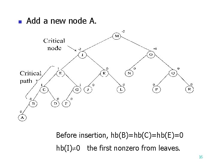
n Add a new node A. Before insertion, hb(B)=hb(C)=hb(E)=0 hb(I) 0 the first nonzero from leaves. 16

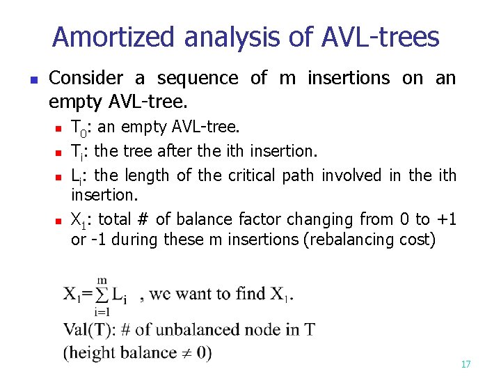
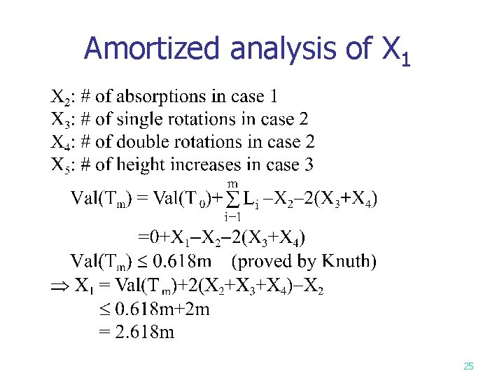
Amortized analysis of AVL-trees n Consider a sequence of m insertions on an empty AVL-tree. n n T 0: an empty AVL-tree. Ti: the tree after the ith insertion. Li: the length of the critical path involved in the ith insertion. X 1: total # of balance factor changing from 0 to +1 or -1 during these m insertions (rebalancing cost) 17

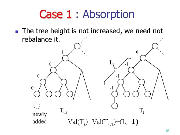
Case 1 : Absorption Case 1 n The tree height is not increased, we need not rebalance it. Val(Ti)=Val(Ti-1)+(Li 1) 18

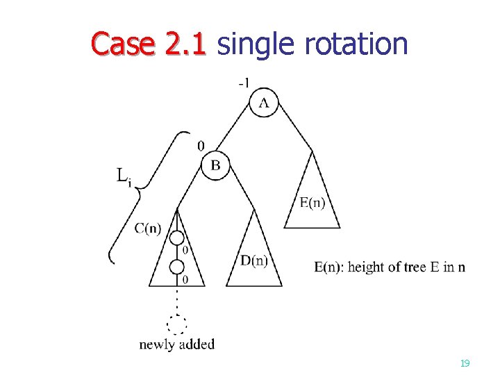
Case 2. 1 single rotation Case 2. 1 19

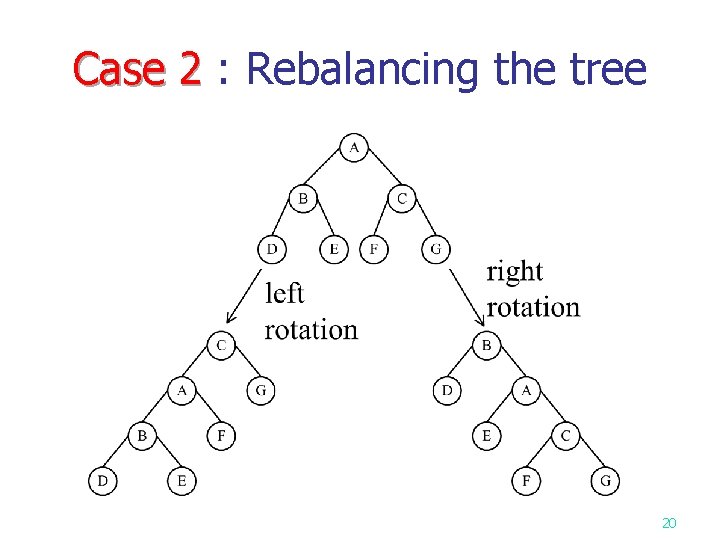
Case 2 : Rebalancing the tree Case 2 20

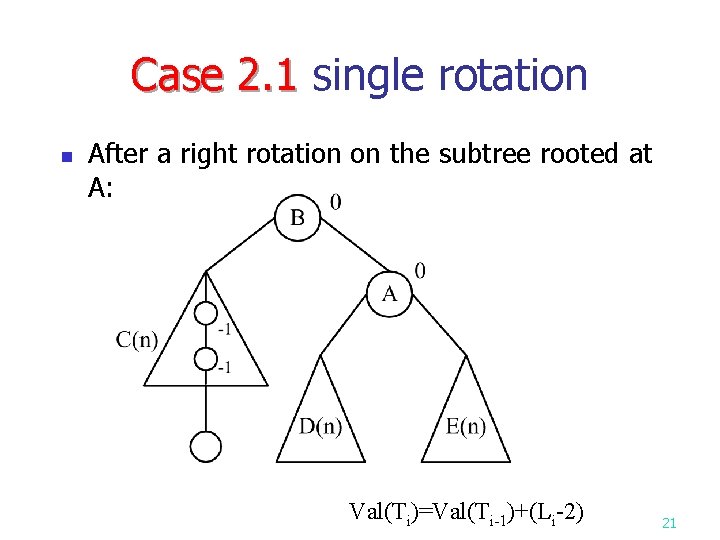
Case 2. 1 single rotation Case 2. 1 n After a right rotation on the subtree rooted at A: Val(Ti)=Val(Ti-1)+(Li-2) 21

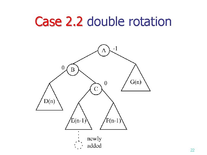
Case 2. 2 double rotation Case 2. 2 22

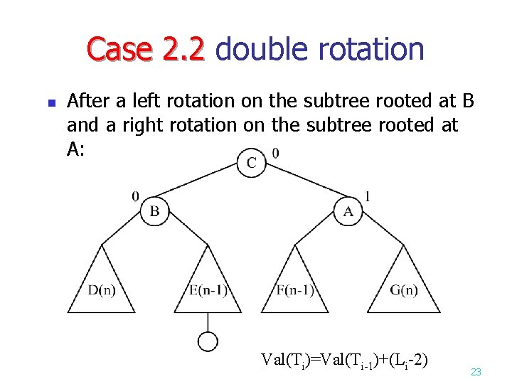
Case 2. 2 double rotation Case 2. 2 n After a left rotation on the subtree rooted at B and a right rotation on the subtree rooted at A: Val(Ti)=Val(Ti-1)+(Li-2) 23

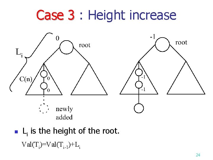
Case 3 : Height increase Case 3 n Li is the height of the root. Val(Ti)=Val(Ti-1)+Li 24

Amortized analysis of X 1 25

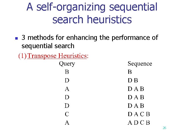
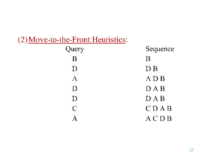
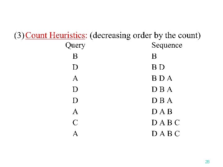
A self-organizing sequential search heuristics n 3 methods for enhancing the performance of sequential search 26

27

28

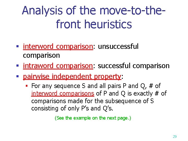
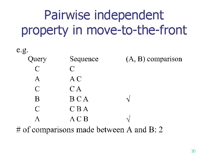
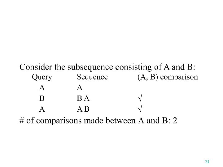
Analysis of the move-to-thefront heuristics § interword comparison: unsuccessful comparison § intraword comparison: successful comparison § pairwise independent property: § For any sequence S and all pairs P and Q, # of interword comparisons of P and Q is exactly # of comparisons made for the subsequence of S consisting of only P’s and Q’s. (See the example on the next page. ) 29

Pairwise independent property in move-to-the-front 30

31

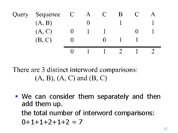
§ We can consider them separately and then add them up. the total number of interword comparisons: 0+1+1+2 = 7 32

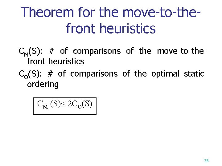
Theorem for the move-to-the- front heuristics CM(S): # of comparisons of the move-to-thefront heuristics CO(S): # of comparisons of the optimal static ordering CM (S) 2 CO(S) 33

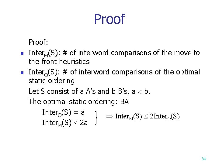
Proof: n Inter. M(S): # of interword comparisons of the move to the front heuristics n Inter. O(S): # of interword comparisons of the optimal static ordering Let S consist of a A’s and b B’s, a b. The optimal static ordering: BA Inter. O(S) = a Inter. M(S) 2 Inter. O(S) Inter. M(S) 2 a 34

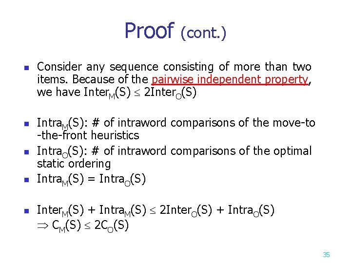
Proof (cont. ) n n n n n Consider any sequence consisting of more than two items. Because of the pairwise independent property, we have Inter. M(S) 2 Inter. O(S) Intra. M(S): # of intraword comparisons of the move-to -the-front heuristics Intra. O(S): # of intraword comparisons of the optimal static ordering Intra. M(S) = Intra. O(S) Inter. M(S) + Intra. M(S) 2 Inter. O(S) + Intra. O(S) CM(S) 2 CO(S) 35

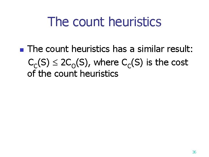
The count heuristics has a similar result: CC(S) 2 CO(S), where CC(S) is the cost of the count heuristics n 36

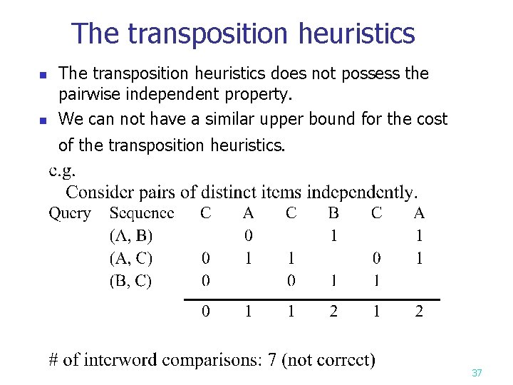
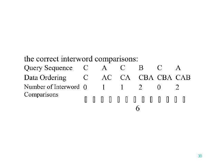
The transposition heuristics n n The transposition heuristics does not possess the pairwise independent property. We can not have a similar upper bound for the cost of the transposition heuristics. 37

38