Tirgul 9 Amortized analysis Graph representation Amortized Analysis

Tirgul 9 • Amortized analysis • Graph representation

Amortized Analysis • Many times we have data structures where some operations take time O(n) in the worst-case. But the total time to perform n operations is less than O(n 2. ( • Amortized analysis is used for exactly such cases. We want to analyze the average time per operation, for the worst sequence of n operations. • So, this is a combination of a worst case analysis with an average case analysis, but without assuming any distribution on the input.

Example - Stack with multi-pop • As a first example we analyze the performance of a stack with one additional operation - multipop(k)- that pops the top k elements of the stack. • Since multipop can take O(n) time in the worst-case, we might conclude that n stack operations can take O(n 2) in the worst case. • We will analyze this simple D. S. using three methods: – The aggregate method – The accounting method – The potential method and see that the average time per operation is still O(1. (

The aggregate method • In this method we find T(n), the total time to perform n operations in the worst-case. The amortized cost of each operation is then defined as T(n)/n • In our stack example, T(n) = O(n) : If we performed a total of k push operations, then the total time for the pop and multipop operations is also at most k (the number of elements we can pop is at most the number of elements we pushed). Since k is at most n, then T(n)=O(n. ( • Thus the amortized cost for all operations is O(1. (

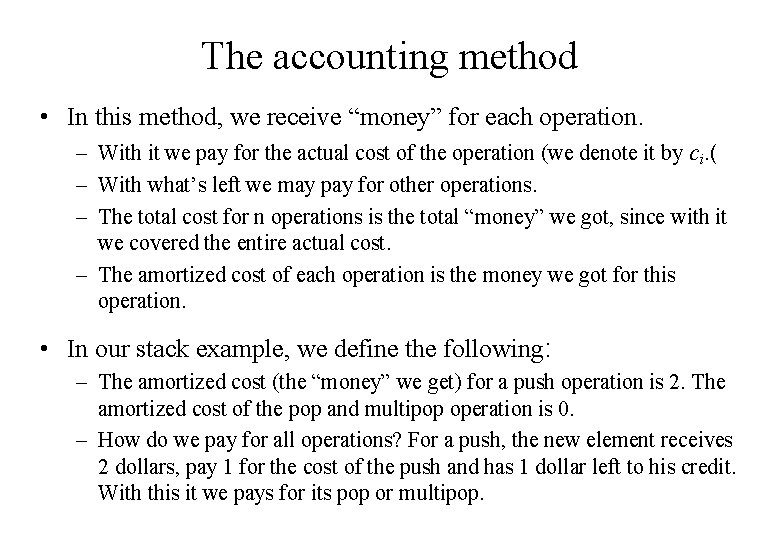
The accounting method • In this method, we receive “money” for each operation. – With it we pay for the actual cost of the operation (we denote it by ci. ( – With what’s left we may pay for other operations. – The total cost for n operations is the total “money” we got, since with it we covered the entire actual cost. – The amortized cost of each operation is the money we got for this operation. • In our stack example, we define the following: – The amortized cost (the “money” we get) for a push operation is 2. The amortized cost of the pop and multipop operation is 0. – How do we pay for all operations? For a push, the new element receives 2 dollars, pay 1 for the cost of the push and has 1 dollar left to his credit. With this it we pays for its pop or multipop.

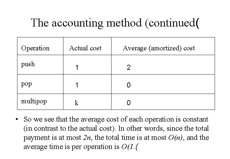
The accounting method (continued( Operation Actual cost Average (amortized) cost push 1 2 pop 1 0 multipop k 0 • So we see that the average cost of each operation is constant (in contrast to the actual cost). In other words, since the total payment is at most 2 n, the total time is at most O(n), and the average time is per operation is O(1. (

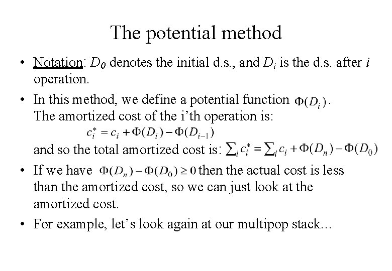
The potential method • Notation: D 0 denotes the initial d. s. , and Di is the d. s. after i operation. • In this method, we define a potential function. The amortized cost of the i’th operation is: and so the total amortized cost is: • If we have then the actual cost is less than the amortized cost, so we can just look at the amortized cost. • For example, let’s look again at our multipop stack. . .

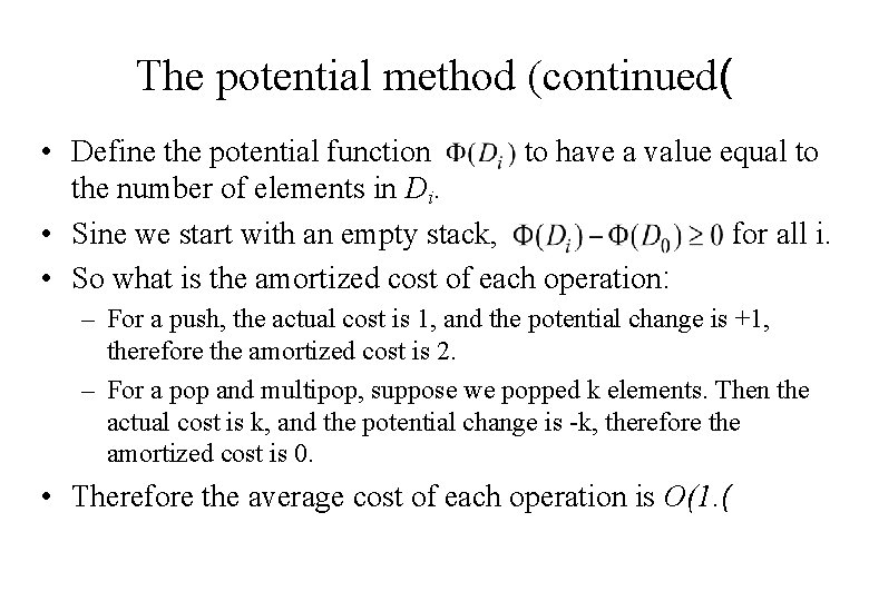
The potential method (continued( • Define the potential function to have a value equal to the number of elements in Di. • Sine we start with an empty stack, for all i. • So what is the amortized cost of each operation: – For a push, the actual cost is 1, and the potential change is +1, therefore the amortized cost is 2. – For a pop and multipop, suppose we popped k elements. Then the actual cost is k, and the potential change is -k, therefore the amortized cost is 0. • Therefore the average cost of each operation is O(1. (

Dynamic Tables • Dynamic table is an array that expands and shrinks dynamically when it becomes over/under-loaded, to fit itself to a variable demand. What is it good for? – Hash tables. – Heaps. – Java’s Vector (if no free cells are left in the middle. ( • In a dynamic table, besides the regular insert and delete, there also: – Expansion: when the table is overloaded and we want to insert a new element. – Contraction: when a delete causes the table to become underloaded. ) the exact meaning of over/under-loaded will be discussed in the next slides. (

Expansion • Our goal: to find the amortized cost of the following expansion operation: – Start with a size of 1. – Upon an insert, if the table is full, create a table twice the old size and copy the old table to beginning of the new one. • Actual cost: 1 for regular insertion, size(T) for expansion. • First intuition to amortized cost, the accounting method: – Suppose we pay 3 for every regular insertion: 1 for the actual cost, and 2 remains as credit for this element. – How do we pay for an expansion? Suppose the table is doubled from size x to 2 x. Then we have x/2 elements that didn’t pay for an expansion yet (have credit of 2). Thus each one of them pays for itself and for one other element out of the x/2 with credit 0.

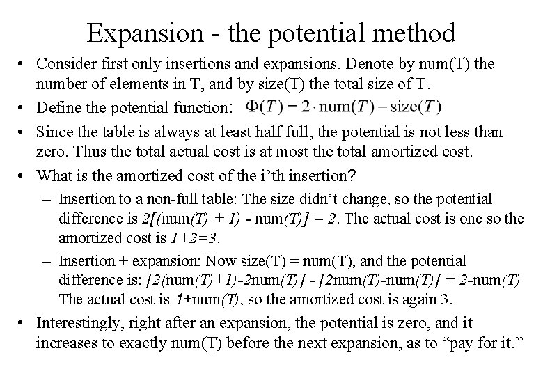
Expansion - the potential method • Consider first only insertions and expansions. Denote by num(T) the number of elements in T, and by size(T) the total size of T. • Define the potential function: • Since the table is always at least half full, the potential is not less than zero. Thus the total actual cost is at most the total amortized cost. • What is the amortized cost of the i’th insertion? – Insertion to a non-full table: The size didn’t change, so the potential difference is 2[(num(T) + 1) - num(T)] = 2. The actual cost is one so the amortized cost is 1+2=3. – Insertion + expansion: Now size(T) = num(T), and the potential difference is: [2(num(T)+1)-2 num(T)] - [2 num(T)-num(T)] = 2 -num(T) The actual cost is 1+num(T), so the amortized cost is again 3. • Interestingly, right after an expansion, the potential is zero, and it increases to exactly num(T) before the next expansion, as to “pay for it. ”

Contraction • Let be the load factor of the table. When it becomes too low, we want to decrease the table size, to save space. • First try: if there are only insertions we are guaranteed that. So, if the load factor decreases below 1/2, decrease the table size by half. • Problem: the amortized cost may be high. For example, suppose a full table with size x, and after one insertion the table expands. Now, after two deletes the table contracts, then after two insertions the table expands again, and so. If we do this many times the average cost per operation will get close to x. • Conclusion: We must ensure that before a contraction, we perform enough operations to pay for it.

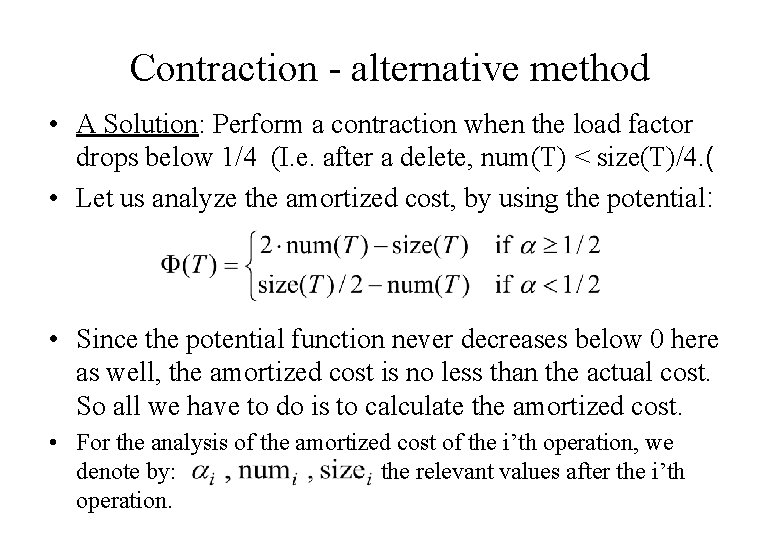
Contraction - alternative method • A Solution: Perform a contraction when the load factor drops below 1/4 (I. e. after a delete, num(T) < size(T)/4. ( • Let us analyze the amortized cost, by using the potential: • Since the potential function never decreases below 0 here as well, the amortized cost is no less than the actual cost. So all we have to do is to calculate the amortized cost. • For the analysis of the amortized cost of the i’th operation, we denote by: the relevant values after the i’th operation.

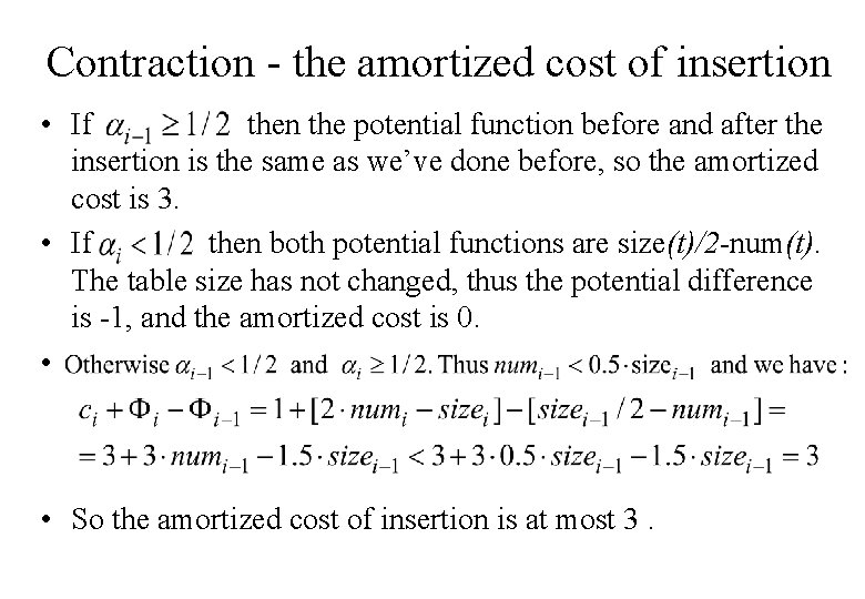
Contraction - the amortized cost of insertion • If then the potential function before and after the insertion is the same as we’ve done before, so the amortized cost is 3. • If then both potential functions are size(t)/2 -num(t). The table size has not changed, thus the potential difference is -1, and the amortized cost is 0. • • So the amortized cost of insertion is at most 3.

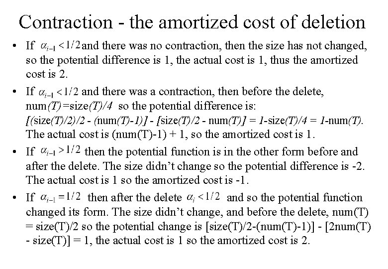
Contraction - the amortized cost of deletion • If and there was no contraction, then the size has not changed, so the potential difference is 1, the actual cost is 1, thus the amortized cost is 2. • If and there was a contraction, then before the delete, num(T)=size(T)/4 so the potential difference is: [(size(T)/2)/2 - (num(T)-1)] - [size(T)/2 - num(T)] = 1 -size(T)/4 = 1 -num(T). The actual cost is (num(T)-1) + 1, so the amortized cost is 1. • If then the potential function is in the other form before and after the delete. The size didn’t change so the potential difference is -2. The actual cost is 1 so the amortized cost is -1. • If then after the delete and so the potential function changed its form. The size didn’t change, and before the delete, num(T) = size(T)/2 so the potential change is [size(T)/2 -(num(T)-1)] - [2 num(T) - size(T)] = 1, the actual cost is 1 so the amortized cost is 2.

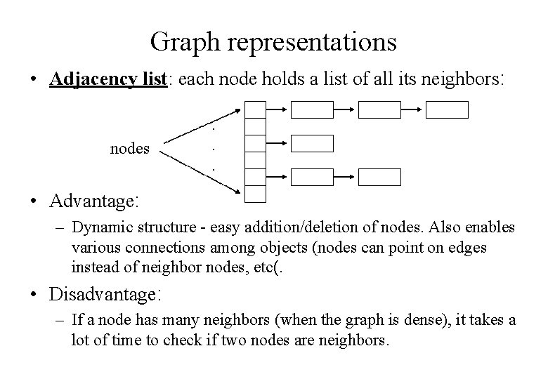
Graph representations • Adjacency list: each node holds a list of all its neighbors: nodes . . . • Advantage: – Dynamic structure - easy addition/deletion of nodes. Also enables various connections among objects (nodes can point on edges instead of neighbor nodes, etc(. • Disadvantage: – If a node has many neighbors (when the graph is dense), it takes a lot of time to check if two nodes are neighbors.

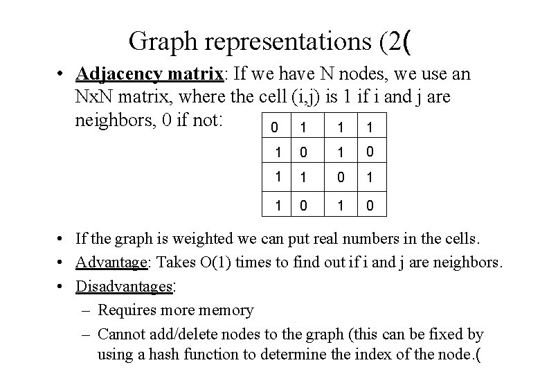
Graph representations (2( • Adjacency matrix: If we have N nodes, we use an Nx. N matrix, where the cell (i, j) is 1 if i and j are neighbors, 0 if not: 0 1 1 0 1 0 • If the graph is weighted we can put real numbers in the cells. • Advantage: Takes O(1) times to find out if i and j are neighbors. • Disadvantages: – Requires more memory – Cannot add/delete nodes to the graph (this can be fixed by using a hash function to determine the index of the node. (

Graph representations (3( • In summary, the considerations for choosing a graph d. s. are: – The needs of the algorithm we intend to use. – Space vs. Time (as usual(. . . – The need to have a dynamic structure.

Sparse matrices • The choice between matrix and list representation is related to sparse matrices: – when we represent a large matrix, if most of its values are 0, we can represent it by linked lists, similarly to the way described below. – Each row and each column are represented by a linked list. We keep only the non zero entries. Each node in the linked list contains a value and an index, thus representing a non-zero entry. • Besides the space reduction, a linked list representation also improves the performance of the matrix operations (add, multiply): We don’t have to go over all the 0 cells, just over the full ones. • For example, how do we multiply matrices when using a linked list representation? • The disadvantage, as for graphs, is that we can’t determine the value of a specific entry in O(1. (