Amortized Analysis chap 17 Not just consider one

Amortized Analysis (chap. 17) • Not just consider one operation, but a sequence of operations on a given data structure. • Average cost over a sequence of operations. • Probabilistic analysis: – Average case running time: average over all possible inputs for one algorithm (operation). – If using probability, called expected running time. • Amortized analysis: – No involvement of probability – Average performance on a sequence of operations, even some operation is expensive. – Guarantee average performance of each operation among the sequence in worst case.

Three Methods of Amortized Analysis • Aggregate analysis: – Total cost of n operations/n, • Accounting method: – – Assign each type of operation an (different) amortized cost overcharge some operations, store the overcharge as credit on specific objects, then use the credit for compensation for some later operations. • Potential method: – Same as accounting method – But store the credit as “potential energy” and as a whole.

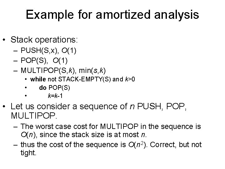
Example for amortized analysis • Stack operations: – PUSH(S, x), O(1) – POP(S), O(1) – MULTIPOP(S, k), min(s, k) • while not STACK-EMPTY(S) and k>0 • do POP(S) • k=k-1 • Let us consider a sequence of n PUSH, POP, MULTIPOP. – The worst case cost for MULTIPOP in the sequence is O(n), since the stack size is at most n. – thus the cost of the sequence is O(n 2). Correct, but not tight.

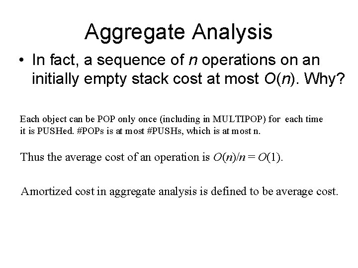
Aggregate Analysis • In fact, a sequence of n operations on an initially empty stack cost at most O(n). Why? Each object can be POP only once (including in MULTIPOP) for each time it is PUSHed. #POPs is at most #PUSHs, which is at most n. Thus the average cost of an operation is O(n)/n = O(1). Amortized cost in aggregate analysis is defined to be average cost.

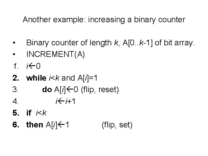
Another example: increasing a binary counter • • 1. 2. 3. 4. 5. 6. Binary counter of length k, A[0. . k-1] of bit array. INCREMENT(A) i 0 while i<k and A[i]=1 do A[i] 0 (flip, reset) i i+1 if i<k then A[i] 1 (flip, set)

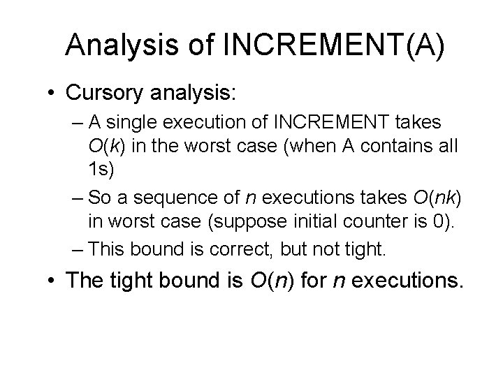
Analysis of INCREMENT(A) • Cursory analysis: – A single execution of INCREMENT takes O(k) in the worst case (when A contains all 1 s) – So a sequence of n executions takes O(nk) in worst case (suppose initial counter is 0). – This bound is correct, but not tight. • The tight bound is O(n) for n executions.

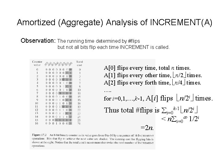
Amortized (Aggregate) Analysis of INCREMENT(A) Observation: The running time determined by #flips but not all bits flip each time INCREMENT is called. A[0] flips every time, total n times. A[1] flips every other time, n/2 times. A[2] flips every forth time, n/4 times. …. for i=0, 1, …, k-1, A[i] flips n/2 i times. Thus total #flips is i=0 k-1 n/2 i < n i=0 1/2 i =2 n.

Amortized Analysis of INCREMENT(A) • Thus the worst case running time is O(n) for a sequence of n INCREMENTs. • So the amortized cost per operation is O(1).

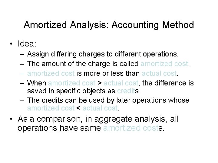
Amortized Analysis: Accounting Method • Idea: – – Assign differing charges to different operations. The amount of the charge is called amortized cost is more or less than actual cost. When amortized cost > actual cost, the difference is saved in specific objects as credits. – The credits can be used by later operations whose amortized cost < actual cost. • As a comparison, in aggregate analysis, all operations have same amortized costs.

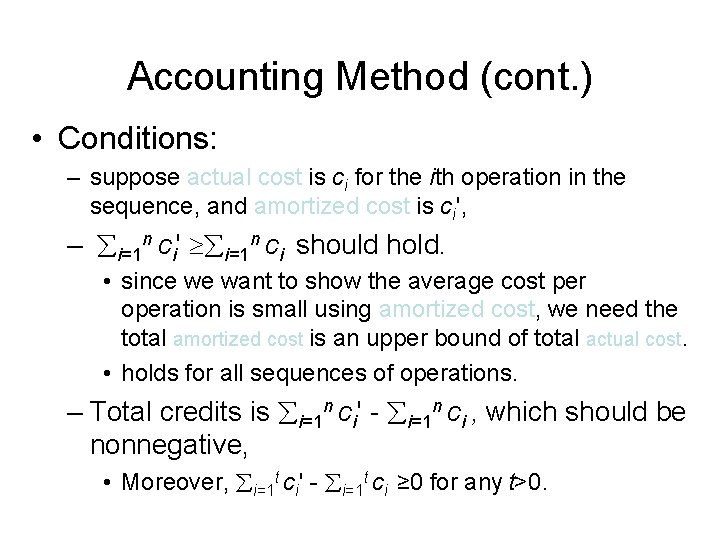
Accounting Method (cont. ) • Conditions: – suppose actual cost is ci for the ith operation in the sequence, and amortized cost is ci', – i=1 n ci' i=1 n ci should hold. • since we want to show the average cost per operation is small using amortized cost, we need the total amortized cost is an upper bound of total actual cost. • holds for all sequences of operations. – Total credits is i=1 n ci' - i=1 n ci , which should be nonnegative, • Moreover, i=1 t ci' - i=1 t ci ≥ 0 for any t>0.

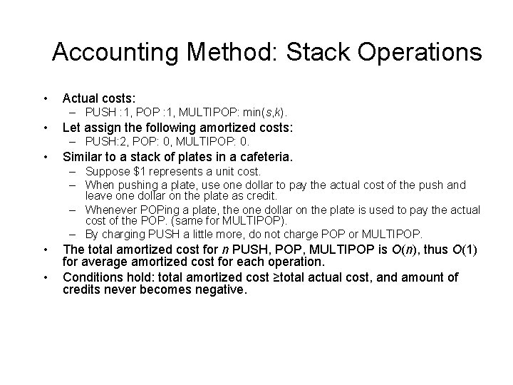
Accounting Method: Stack Operations • Actual costs: – PUSH : 1, POP : 1, MULTIPOP: min(s, k). • Let assign the following amortized costs: – PUSH: 2, POP: 0, MULTIPOP: 0. • Similar to a stack of plates in a cafeteria. – Suppose $1 represents a unit cost. – When pushing a plate, use one dollar to pay the actual cost of the push and leave one dollar on the plate as credit. – Whenever POPing a plate, the one dollar on the plate is used to pay the actual cost of the POP. (same for MULTIPOP). – By charging PUSH a little more, do not charge POP or MULTIPOP. • • The total amortized cost for n PUSH, POP, MULTIPOP is O(n), thus O(1) for average amortized cost for each operation. Conditions hold: total amortized cost ≥total actual cost, and amount of credits never becomes negative.

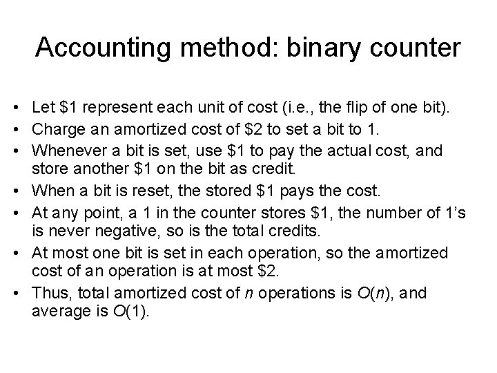
Accounting method: binary counter • Let $1 represent each unit of cost (i. e. , the flip of one bit). • Charge an amortized cost of $2 to set a bit to 1. • Whenever a bit is set, use $1 to pay the actual cost, and store another $1 on the bit as credit. • When a bit is reset, the stored $1 pays the cost. • At any point, a 1 in the counter stores $1, the number of 1’s is never negative, so is the total credits. • At most one bit is set in each operation, so the amortized cost of an operation is at most $2. • Thus, total amortized cost of n operations is O(n), and average is O(1).

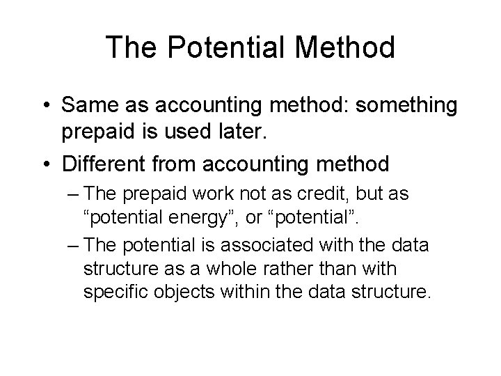
The Potential Method • Same as accounting method: something prepaid is used later. • Different from accounting method – The prepaid work not as credit, but as “potential energy”, or “potential”. – The potential is associated with the data structure as a whole rather than with specific objects within the data structure.

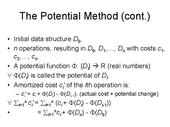
The Potential Method (cont. ) • Initial data structure D 0, • n operations, resulting in D 0, D 1, …, Dn with costs c 1, c 2, …, cn. • A potential function : {Di} R (real numbers) (Di) is called the potential of Di. • Amortized cost ci' of the ith operation is: – ci' = ci + (Di) - (Di-1). (actual cost + potential change) i=1 n ci' = i=1 n (ci + (Di) - (Di-1)) • = i=1 nci + (Dn) - (D 0)

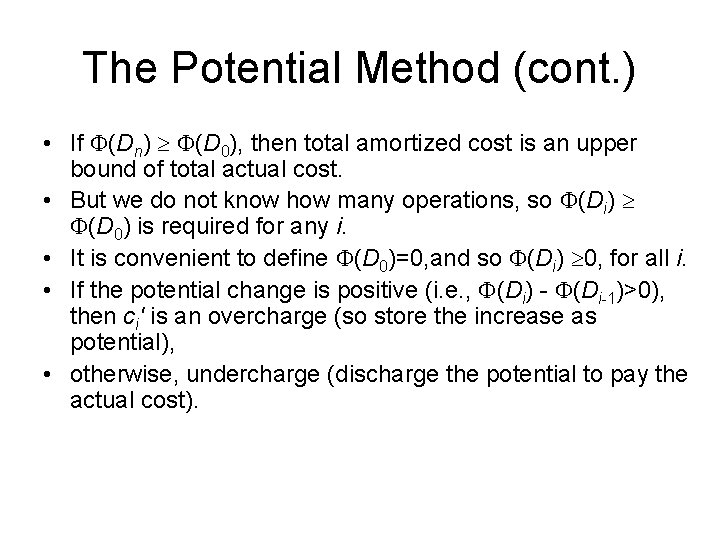
The Potential Method (cont. ) • If (Dn) (D 0), then total amortized cost is an upper bound of total actual cost. • But we do not know how many operations, so (Di) (D 0) is required for any i. • It is convenient to define (D 0)=0, and so (Di) 0, for all i. • If the potential change is positive (i. e. , (Di) - (Di-1)>0), then ci' is an overcharge (so store the increase as potential), • otherwise, undercharge (discharge the potential to pay the actual cost).

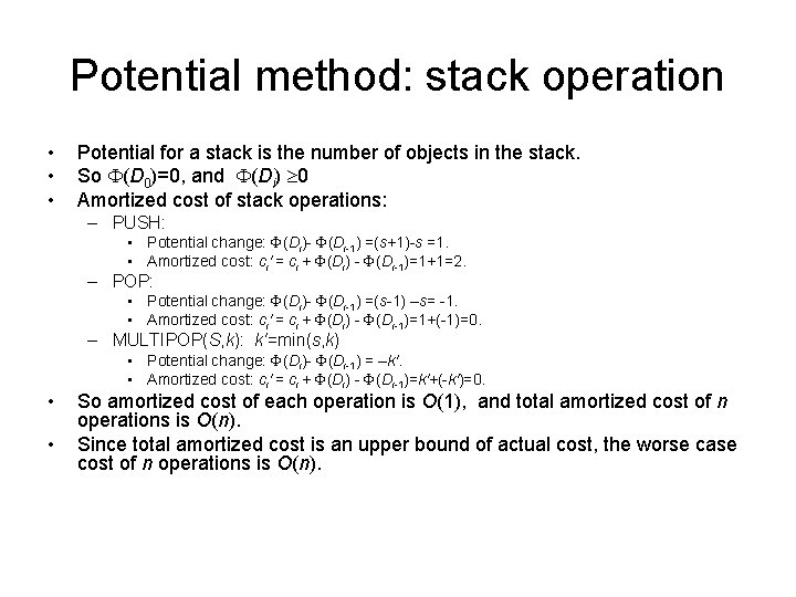
Potential method: stack operation • • • Potential for a stack is the number of objects in the stack. So (D 0)=0, and (Di) 0 Amortized cost of stack operations: – PUSH: • Potential change: (Di)- (Di-1) =(s+1)-s =1. • Amortized cost: ci' = ci + (Di) - (Di-1)=1+1=2. – POP: • Potential change: (Di)- (Di-1) =(s-1) –s= -1. • Amortized cost: ci' = ci + (Di) - (Di-1)=1+(-1)=0. – MULTIPOP(S, k): k'=min(s, k) • • • Potential change: (Di)- (Di-1) = –k'. • Amortized cost: ci' = ci + (Di) - (Di-1)=k'+(-k')=0. So amortized cost of each operation is O(1), and total amortized cost of n operations is O(n). Since total amortized cost is an upper bound of actual cost, the worse case cost of n operations is O(n).

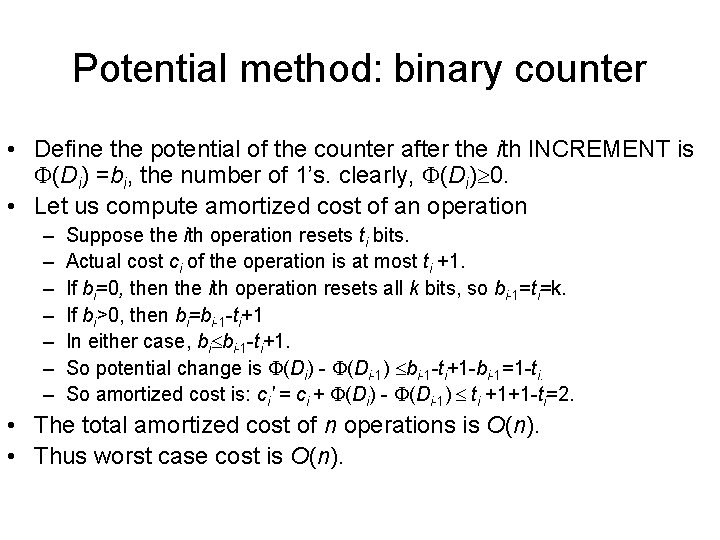
Potential method: binary counter • Define the potential of the counter after the ith INCREMENT is (Di) =bi, the number of 1’s. clearly, (Di) 0. • Let us compute amortized cost of an operation – – – – Suppose the ith operation resets ti bits. Actual cost ci of the operation is at most ti +1. If bi=0, then the ith operation resets all k bits, so bi-1=ti=k. If bi>0, then bi=bi-1 -ti+1 In either case, bi bi-1 -ti+1. So potential change is (Di) - (Di-1) bi-1 -ti+1 -bi-1=1 -ti. So amortized cost is: ci' = ci + (Di) - (Di-1) ti +1+1 -ti=2. • The total amortized cost of n operations is O(n). • Thus worst case cost is O(n).

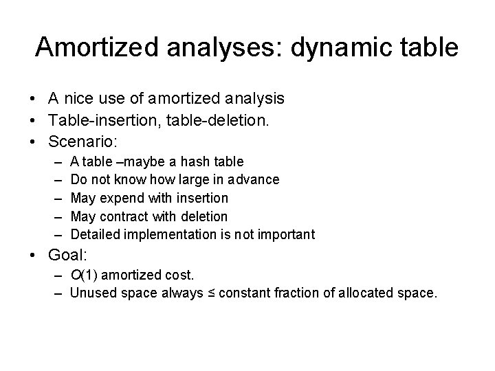
Amortized analyses: dynamic table • A nice use of amortized analysis • Table-insertion, table-deletion. • Scenario: – – – A table –maybe a hash table Do not know how large in advance May expend with insertion May contract with deletion Detailed implementation is not important • Goal: – O(1) amortized cost. – Unused space always ≤ constant fraction of allocated space.

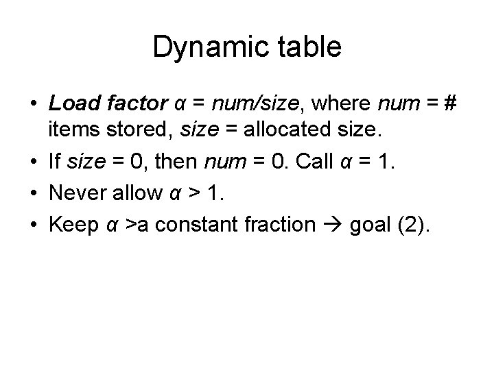
Dynamic table • Load factor α = num/size, where num = # items stored, size = allocated size. • If size = 0, then num = 0. Call α = 1. • Never allow α > 1. • Keep α >a constant fraction goal (2).

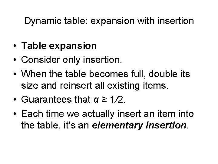
Dynamic table: expansion with insertion • Table expansion • Consider only insertion. • When the table becomes full, double its size and reinsert all existing items. • Guarantees that α ≥ 1/2. • Each time we actually insert an item into the table, it’s an elementary insertion.

Copyright © The Mc. Graw-Hill Companies, Inc. Permission required for reproduction or display. Num[t] ele. insertion 1 ele. insertion Initially, num[T ] = size[T ] = 0.

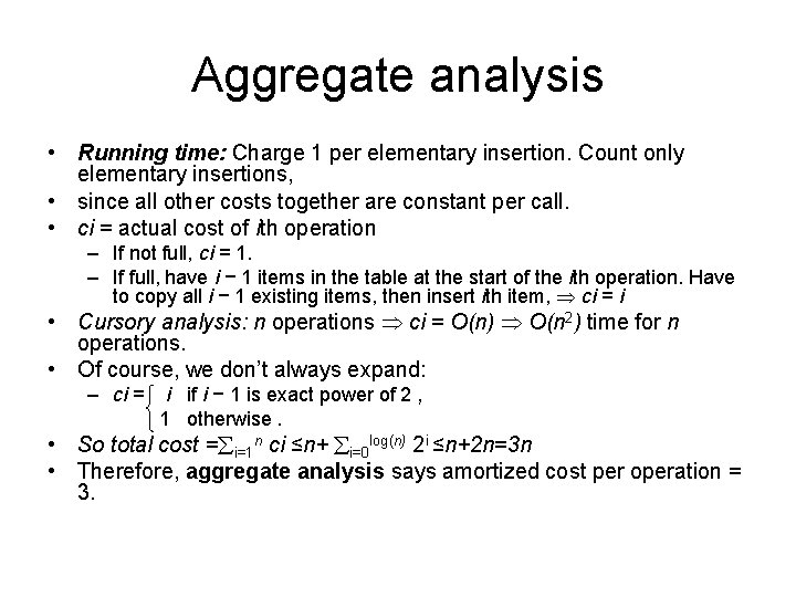
Aggregate analysis • Running time: Charge 1 per elementary insertion. Count only elementary insertions, • since all other costs together are constant per call. • ci = actual cost of ith operation – If not full, ci = 1. – If full, have i − 1 items in the table at the start of the ith operation. Have to copy all i − 1 existing items, then insert ith item, ci = i • Cursory analysis: n operations ci = O(n) O(n 2) time for n operations. • Of course, we don’t always expand: – ci = i if i − 1 is exact power of 2 , 1 otherwise. • So total cost = i=1 n ci ≤n+ i=0 log(n) 2 i ≤n+2 n=3 n • Therefore, aggregate analysis says amortized cost per operation = 3.

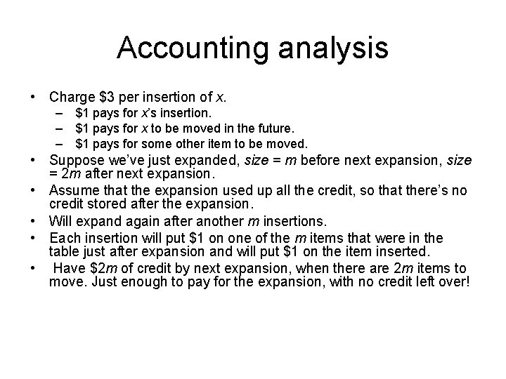
Accounting analysis • Charge $3 per insertion of x. – $1 pays for x’s insertion. – $1 pays for x to be moved in the future. – $1 pays for some other item to be moved. • Suppose we’ve just expanded, size = m before next expansion, size = 2 m after next expansion. • Assume that the expansion used up all the credit, so that there’s no credit stored after the expansion. • Will expand again after another m insertions. • Each insertion will put $1 on one of the m items that were in the table just after expansion and will put $1 on the item inserted. • Have $2 m of credit by next expansion, when there are 2 m items to move. Just enough to pay for the expansion, with no credit left over!

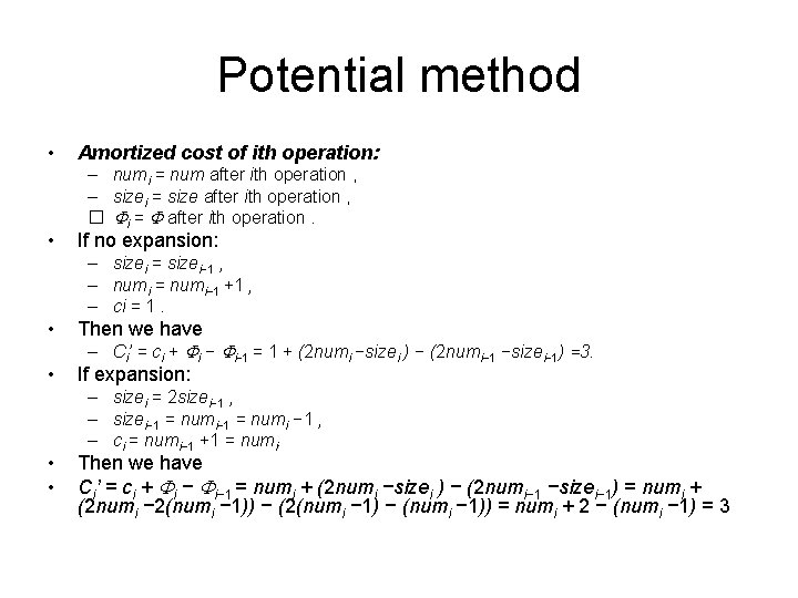
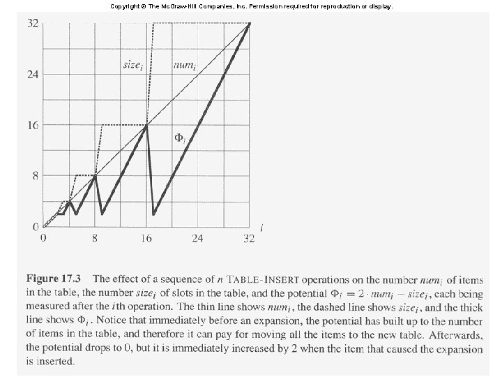
Potential method • Potential method (T ) = 2 ・ num[T ] − size[T ] • Initially, num = size = 0. • • Just after expansion, size = 2 ・ num = 0. • Just before expansion, size = num have enough potential to pay for moving all items. • Need ≥ 0, always. • Always have – size ≥ num ≥ ½ size 2 ・ num ≥ size ≥ 0.

Potential method • • Amortized cost of ith operation: – numi = num after ith operation , – sizei = size after ith operation , � i = after ith operation. If no expansion: – sizei = sizei− 1 , – numi = numi− 1 +1 , – ci = 1. • Then we have • If expansion: • • – Ci’ = ci + i − i− 1 = 1 + (2 numi −sizei ) − (2 numi− 1 −sizei− 1) =3. – sizei = 2 sizei− 1 , – sizei− 1 = numi − 1 , – ci = numi− 1 +1 = numi. Then we have Ci’ = ci + i − i− 1 = numi + (2 numi −sizei ) − (2 numi− 1 −sizei− 1) = numi + (2 numi − 2(numi − 1)) − (2(numi − 1) − (numi − 1)) = numi + 2 − (numi − 1) = 3

Copyright © The Mc. Graw-Hill Companies, Inc. Permission required for reproduction or display.

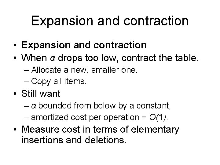
Expansion and contraction • When α drops too low, contract the table. – Allocate a new, smaller one. – Copy all items. • Still want – α bounded from below by a constant, – amortized cost per operation = O(1). • Measure cost in terms of elementary insertions and deletions.

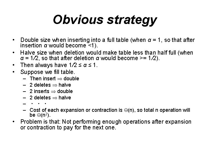
Obvious strategy • Double size when inserting into a full table (when α = 1, so that after insertion α would become <1). • Halve size when deletion would make table less than half full (when α = 1/2, so that after deletion α would become >= 1/2). • Then always have 1/2 ≤ α ≤ 1. • Suppose we fill table. – – – Then insert double 2 deletes halve 2 inserts double 2 deletes halve ・・・ Cost of each expansion or contraction is (n), so total n operation will be (n 2). • Problem is that: Not performing enough operations after expansion or contraction to pay for the next one.

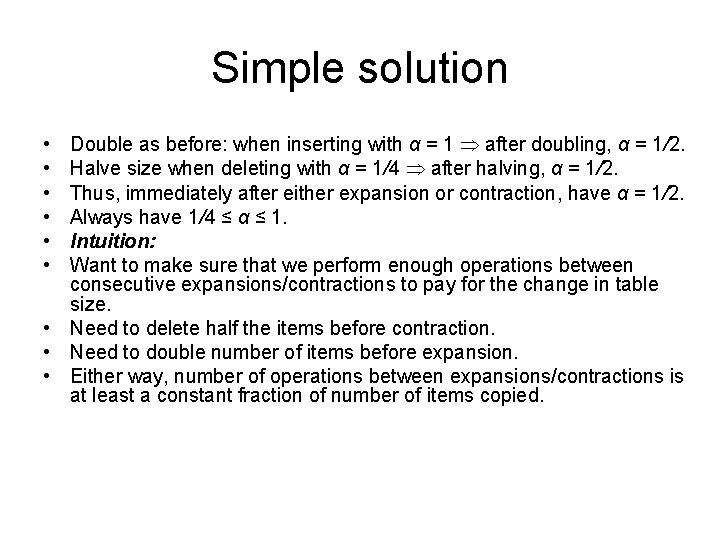
Simple solution Double as before: when inserting with α = 1 after doubling, α = 1/2. Halve size when deleting with α = 1/4 after halving, α = 1/2. Thus, immediately after either expansion or contraction, have α = 1/2. Always have 1/4 ≤ α ≤ 1. Intuition: Want to make sure that we perform enough operations between consecutive expansions/contractions to pay for the change in table size. • Need to delete half the items before contraction. • Need to double number of items before expansion. • Either way, number of operations between expansions/contractions is at least a constant fraction of number of items copied. • • •

Potential function (T) = 2 num[T] − size[T] if α ≥ ½ size[T]/2 −num[T] ifα < ½. • T empty = 0. • α ≥ 1/2 num ≥ 1/2 size 2 num ≥ size ≥ 0. • α < 1/2 num < 1/2 size ≥ 0.

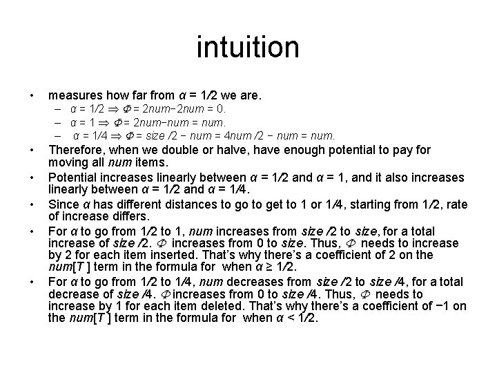
intuition • measures how far from α = 1/2 we are. • Therefore, when we double or halve, have enough potential to pay for moving all num items. Potential increases linearly between α = 1/2 and α = 1, and it also increases linearly between α = 1/2 and α = 1/4. Since α has different distances to go to get to 1 or 1/4, starting from 1/2, rate of increase differs. For α to go from 1/2 to 1, num increases from size /2 to size, for a total increase of size /2. increases from 0 to size. Thus, needs to increase by 2 for each item inserted. That’s why there’s a coefficient of 2 on the num[T ] term in the formula for when α ≥ 1/2. For α to go from 1/2 to 1/4, num decreases from size /2 to size /4, for a total decrease of size /4. increases from 0 to size /4. Thus, needs to increase by 1 for each item deleted. That’s why there’s a coefficient of − 1 on the num[T ] term in the formula for when α < 1/2. • • – α = 1/2 = 2 num− 2 num = 0. – α = 1 = 2 num−num = num. – α = 1/4 = size /2 − num = 4 num /2 − num = num.

Amortized cost for each operation • Amortized costs: more cases – insert, delete – α ≥ 1/2, α < 1/2 (use αi, since α can vary a lot) – size does/doesn’t change

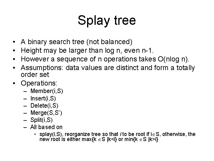
Splay tree • • A binary search tree (not balanced) Height may be larger than log n, even n-1. However a sequence of n operations takes O(nlog n). Assumptions: data values are distinct and form a totally order set • Operations: – – – Member(i, S) Insert(i, S) Delete(i, S) Merge(S, S’) Split(i, S) All based on • splay(i, S), reorganize tree so that i to be root if i S, otherwise, the new root is either max{k S |k<i} or min{k S |k>i}

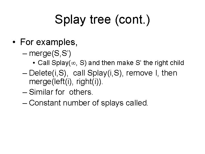
Splay tree (cont. ) • For examples, – merge(S, S’) • Call Splay( , S) and then make S’ the right child – Delete(i, S), call Splay(i, S), remove I, then merge(left(i), right(i)). – Similar for others. – Constant number of splays called.

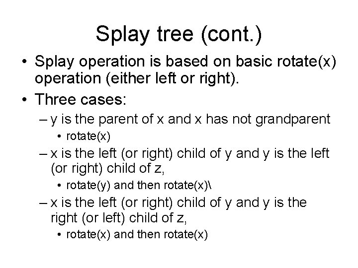
Splay tree (cont. ) • Splay operation is based on basic rotate(x) operation (either left or right). • Three cases: – y is the parent of x and x has not grandparent • rotate(x) – x is the left (or right) child of y and y is the left (or right) child of z, • rotate(y) and then rotate(x) – x is the left (or right) child of y and y is the right (or left) child of z, • rotate(x) and then rotate(x)

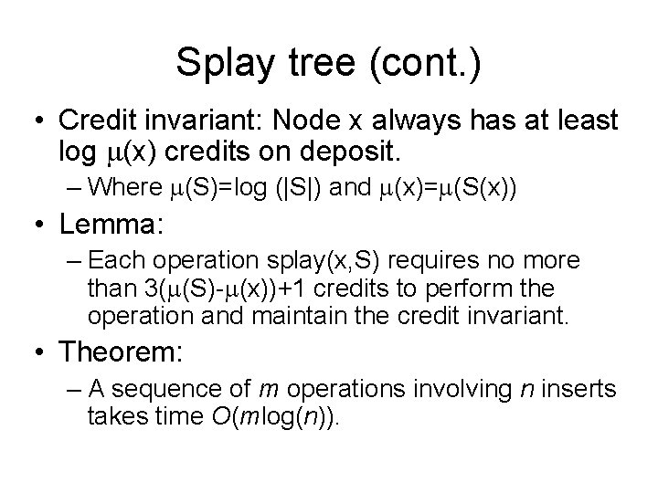
Splay tree (cont. ) • Credit invariant: Node x always has at least log (x) credits on deposit. – Where (S)=log (|S|) and (x)= (S(x)) • Lemma: – Each operation splay(x, S) requires no more than 3( (S)- (x))+1 credits to perform the operation and maintain the credit invariant. • Theorem: – A sequence of m operations involving n inserts takes time O(mlog(n)).

Summary • Amortized analysis – Different from probabilistic analysis • Three methods and their differences • how to analyze