Chapter 5 Geometric Transformations Push versus Pull Push

Chapter 5: Geometric Transformations

Push versus Pull Push: uses the source pixels to control the computation process Pull: uses the destination pixels to control the computation process Example: Add 10 to each pixel value in the source image to produce the corresponding value in the destination image 25 11 26 27 35 21 36 37 28 22 20 24 38 32 30 34 25 21 22 23 35 31 32 33 29 27 19 26 39 37 29 36 source image destination image

Push versus Pull Are push and pull the same? What is the advantage of one over the other? Example: Using PUSH, double the size of the image Destination(x*2, y*2) = Source(x, y) 35 - 21 - 36 - 37 - - - - - 25 11 26 27 28 22 20 24 38 - 32 - 30 - 34 - 25 21 22 23 - - - - 29 27 19 26 35 - 31 32 - 33 - - - - destination 39 image - - 37 29 - 36 - - - - source image -

Push versus Pull Are push and pull the same? What is the advantage of one over the other? Example: Using PULL, double the size of the image Destination(x, y) = Source(x/2, y/2) 35 35 21 21 36 36 37 37 25 11 26 27 35 35 21 21 36 36 37 37 28 22 20 24 38 38 32 32 30 30 34 34 25 21 22 23 38 38 32 32 30 30 34 34 29 27 19 26 35 35 31 31 32 32 33 33 destination 39 image 39 39 37 37 29 29 36 36 source image

Spatial Transformations - translation - reflection - scaling - rotation in 90 degree increments - rotation at an arbitrary angle - perspective transformations - image registration - warping / morphing

Geometric Transformations More complex transformations consist of two basic operations: (1) a spatial transformation - defines the “rearrangement” of pixels on the image plane (2) a grey-level interpolation method - determines the assignment of intensity values to pixels in the spatially transformed image

Interpolation Methods: - nearest neighbor - bilinear interpolation - cubic B-spline

Interpolation Methods: NEAREST NEIGHBOR (zero-order interpolation) : assigns pixel value to that of nearest neighbor advantages: - simple and efficient implementation - enables image zooming disadvantages: - may produce distortion of edges - undesirable sawtooth artifacts (jaggies)

Interpolation Methods: BILINEAR INTERPOLATION (first-order interpolation) : assigns pixel value as a weighted interpolation of the values of its four defined neighbors advantages: - relatively simple and efficient - produces more desirable (smoother) results than nearest neighbor disadvantages: - derivatives of piecewise bilinear surfaces are discontinuous at neighborhood boundaries

Interpolation Methods: CUBIC B-SPLINE (third-order interpolation) : assigns pixel value as a weighted interpolation of the values of a larger set of defined neighbors advantages: - produces most desirable (smoothest) results disadvantages: - computationally costly

Geometric Transformations - Example: SCALING (1) a spatial transformation: ’ X = S x X, ’ Y = Sy Y (2) a grey-level interpolation method - nearest neighbor (pixel replication) bilinear interpolation (average of 4 neighbors) cubic b-spline

Geometric Transformations: Power of two SCALING When Sx = Sy = 2 k, all three methods of grey level interpolation may be performed by 1) inserting zero values into image for every other row and every other column 2) performing a convolution with the proper convolution kernel

Geometric Transformations: Convolution Values in an image are multiplied by corresponding locations in a “kernel” and the results of those multiplications are summed to produce the resulting pixel in a new image. Original image Zoomed image

Geometric Transformations: Convolution Values in an image are multiplied by corresponding locations in a “kernel” and the results of those multiplications are summed to produce the resulting pixel in a new image.

Nearest neighbor * 2 X 1 1

Nearest neighbor 4 X

Bilinear Interpolation * 2 X 1 4 1 2 4 2 1

Bilinear Interpolation 4 X

Cubic B-Spline * 1 64 2 X 1 4 6 4 16 24 16 4 6 24 36 24 6 4 16 24 16 4 1 4 6 4 1

Cubic B-Spline 4 X

Nearest Neighbor Bilinear Interpolation

Bilinear Interpolation Bi-cubic Spline Interpolation

Geometric Transformations: SCALING When Sx = Sy = 2 k, the computation of pixel values for the new image is more complex. Two different schemes are possible for mapping pixel locations from the source image to pixel locations within the new resized image 1) Source-to-target mapping 2) Target-to-source mapping

Geometric Transformations: SCALING When Sx = Sy = 2 k, the computation of pixel values for the new image is more complex. 1) Source-to-target mapping X ’ = SX X, Y ’= S y Y Using this mapping certain pixels in the new image will have nothing mapped to it.

Geometric Transformations: SCALING ’ ’ X = S X, Y =S Y X y With a scaling factor Sx=3, Sy=3 pixel(3, 5) -> newpixel(9, 15) pixel(4, 5) -> newpixel(12, 15) 2 3 4 5 6 7 7 4 14 5 15 6 16 7 17 8 18 9 19 8 9 10 11 12

Geometric Transformations: SCALING ’ ’ X = S X, Y =S Y X y With a source-to-target mapping how does newpixel(10, 15) get its value? 2 3 4 5 6 7 7 4 14 5 15 6 16 7 17 8 18 9 19 8 9 10 11 12

Geometric Transformations: SCALING When Sx = Sy = 2 k, the computation of pixel values for the new image is more complex. 1) Source-to-target mapping 2) Target-to-source mapping ’ S X, X = Y =S Y X X = X / S , ’ ’ y Y = Y/S X ’ y

Geometric Transformations: SCALING X = X / S , ’ ’ Y = Y/S X y With a scaling factor Sx=3, Sy=3 newpixel(9, 15) -> pixel(3, 5) newpixel(10, 15) -> pixel(3. 3, 5) 2 3 4 5 6 7 7 4 14 5 15 6 16 7 17 8 18 9 19 8 9 10 11 12

Geometric Transformations: SCALING newpixel(10, 15) -> pixel(3. 3, 5) 2 4 5 6 7 8 9 3 4 5 6 7 ? ? 1) nearest neighbor round the x, y values and take the new pixel value from that location in the source image 2) bilinear interpolation compute the new pixel value as a weighted average of the neighboring pixels in the source image

Geometric Transformations: - translation - reflection - scaling - rotation in 90 degree increments - rotation at an arbitrary angle - perspective transformations - image registration - warping / morphing

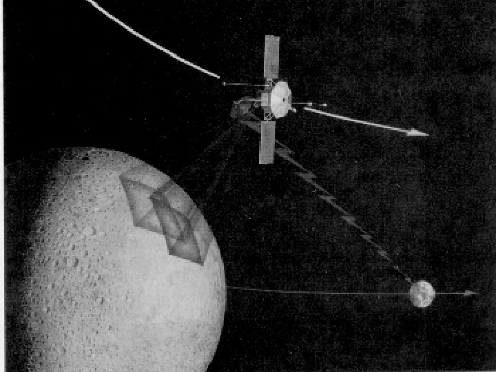
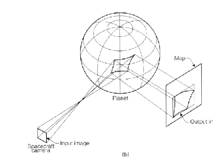
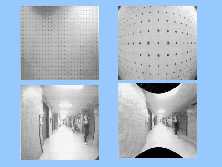
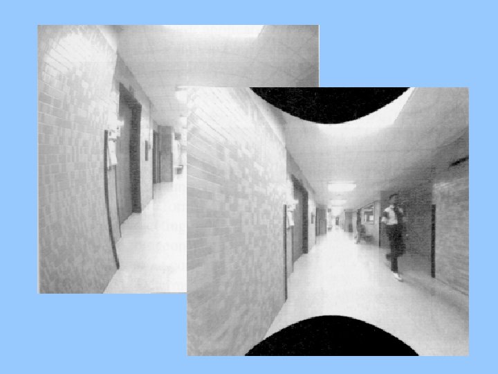
perspective transformations

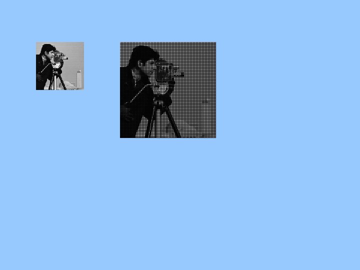
Perspective Transformations Tie points are identified in each image to compute a transformation matrix which can be used to compute remapping locations in the new image

perspective transformations

Calibration images can be used to automate tie point identification