Chapter 1 Lecture Kinematics Motion in One Dimension

Chapter 1 Lecture Kinematics: Motion in One Dimension © 2014 Pearson Education, Inc.

1. 1 What is Motion? © 2014 Pearson Education, Inc.

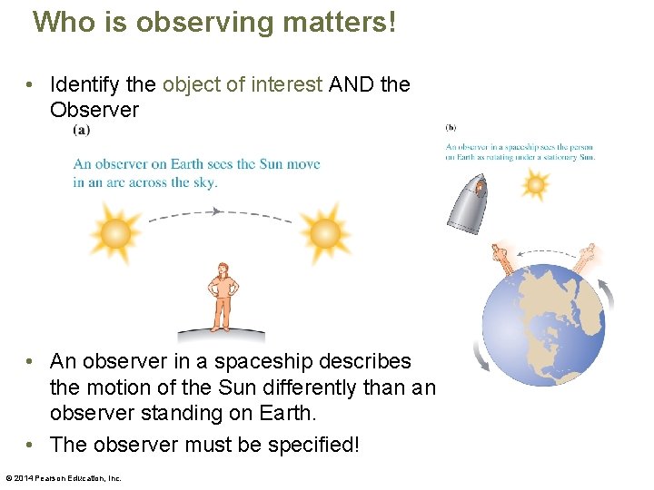
Who is observing matters! • Identify the object of interest AND the Observer • An observer in a spaceship describes the motion of the Sun differently than an observer standing on Earth. • The observer must be specified! © 2014 Pearson Education, Inc.

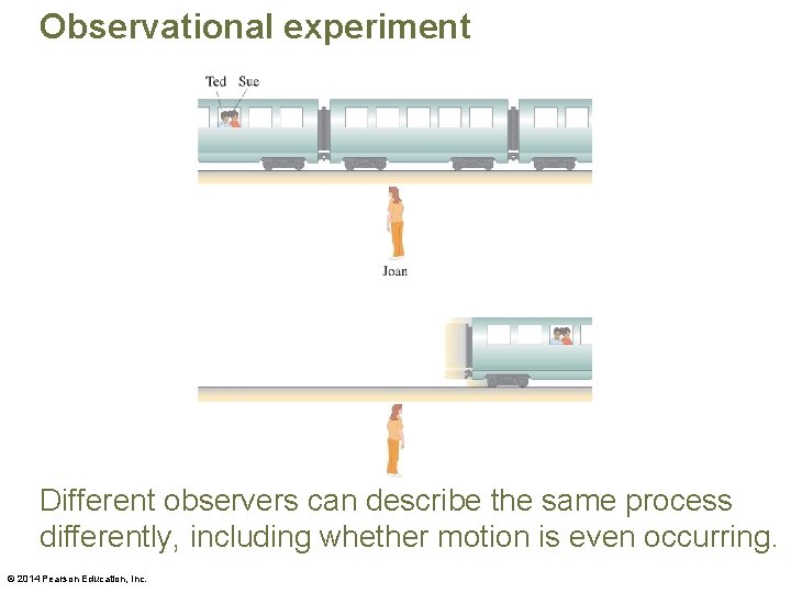
Observational experiment Different observers can describe the same process differently, including whether motion is even occurring. © 2014 Pearson Education, Inc.

1. 2 A Conceptual Description of Motion © 2014 Pearson Education, Inc.

1. 3 Quantities for Describing Motion © 2014 Pearson Education, Inc.

Quantities for describing motion • Motion diagrams represent motion qualitatively. • The quantities needed to describe linear motion: – Time and time interval – Position, displacement, distance, and path length – Scalar component of displacement for motion along one axis © 2014 Pearson Education, Inc.

Time and time interval • The time t is a clock reading. • The time interval (t 2 - t 1) or Δt is a difference in clock readings. (The symbol delta represents "change in" and is the final value minus the initial value. ) • These are both scalar quantities. • The SI units for both quantities are seconds (s). © 2014 Pearson Education, Inc.

Position, displacement, distance, and path length, • These quantities describe the location and motion of an object. – Position is an object's location with respect to a particular coordinate system. – Displacement is a vector that starts from an object's initial position and ends at its final position. – Distance (confusing) 1. the magnitude (length) of the displacement vector or 2. total distance traveled. – Path length is another name for total distance traveled. © 2014 Pearson Education, Inc.

Uniform Motion (CVPM) and (CAPM) • Uniform Motion: motion at a constant velocity (i. e constant velocity and speed (CVPM -constant velocity particle motion) • Uniform Acceleration: motion at a constant acceleration (CAPM-Constant acceleration particle model) (later on this) © 2014 Pearson Education, Inc.

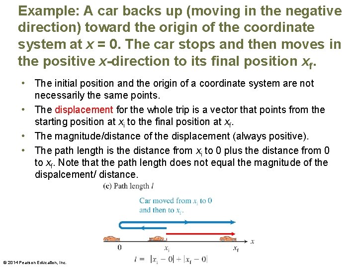
Example: A car backs up (moving in the negative direction) toward the origin of the coordinate system at x = 0. The car stops and then moves in the positive x-direction to its final position xf. • The initial position and the origin of a coordinate system are not necessarily the same points. • The displacement for the whole trip is a vector that points from the starting position at xi to the final position at xf. • The magnitude/distance of the displacement (always positive). • The path length is the distance from xi to 0 plus the distance from 0 to xf. Note that the path length does not equal the magnitude of the dispalcement/ distance. © 2014 Pearson Education, Inc.

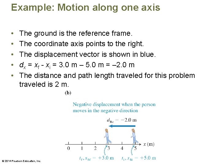
Example: Motion along one axis • • • The ground is the reference frame. The coordinate axis points to the right. The displacement vector is shown in blue. dx = xf - xi = 3. 0 m – 5. 0 m = – 2. 0 m The distance and path length traveled for this problem traveled is 2 m. © 2014 Pearson Education, Inc.

1. 4 The Position Time Plot (P-T) © 2014 Pearson Education, Inc.

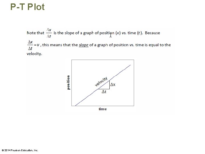
Representing motion with data tables and graphs • A data table records position and time data when observing motion. • A graph of the data in the table can help identify patterns in the data. • This type of graph is called a kinematics position-versus-time graph (P-T graph). • Kinematics means "description of motion. " © 2014 Pearson Education, Inc.

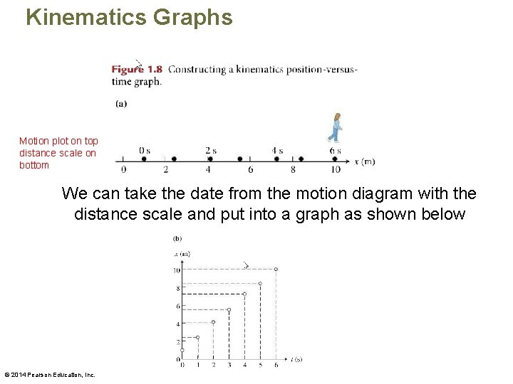
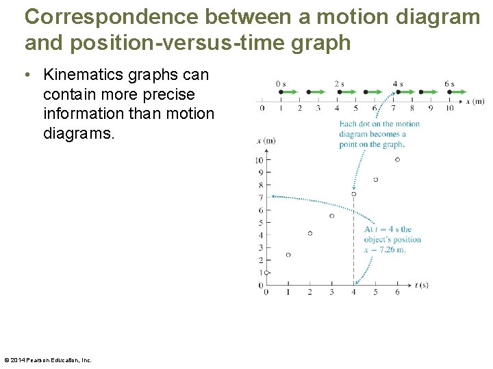
Kinematics Graphs Motion plot on top distance scale on bottom We can take the date from the motion diagram with the distance scale and put into a graph as shown below © 2014 Pearson Education, Inc.

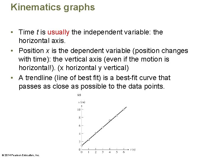
Kinematics graphs • Time t is usually the independent variable: the horizontal axis. • Position x is the dependent variable (position changes with time): the vertical axis (even if the motion is horizontal!). (x horizontal y vertical) • A trendline (line of best fit) is a best-fit curve that passes as close as possible to the data points. © 2014 Pearson Education, Inc.

P-T Plot © 2014 Pearson Education, Inc.

Correspondence between a motion diagram and position-versus-time graph • Kinematics graphs can contain more precise information than motion diagrams. © 2014 Pearson Education, Inc.

P-T Graph • Please understand – Just because the position of the object is being graphed on the vertical axis does NOT MEAN the object is moving vertically!!!!! – This graph is position vs time. P-T graphs can only plot one dimension at time. You would have to 2 P-T graphs if the object was moving horizontally and vertically!!!!! © 2014 Pearson Education, Inc.

1. 5 Constant Velocity Linear Motion (CVPM) P means Particle © 2014 Pearson Education, Inc.

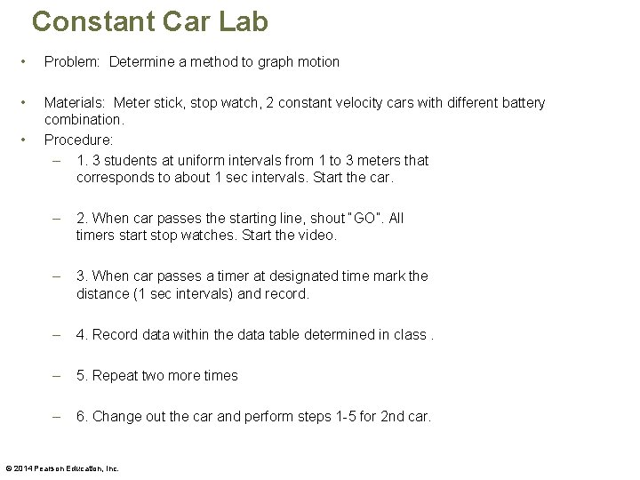
Constant Car Lab • Problem: Determine a method to graph motion • Materials: Meter stick, stop watch, 2 constant velocity cars with different battery combination. Procedure: – 1. 3 students at uniform intervals from 1 to 3 meters that corresponds to about 1 sec intervals. Start the car. • – 2. When car passes the starting line, shout “GO”. All timers start stop watches. Start the video. – 3. When car passes a timer at designated time mark the distance (1 sec intervals) and record. – 4. Record data within the data table determined in class. – 5. Repeat two more times – 6. Change out the car and perform steps 1 -5 for 2 nd car. © 2014 Pearson Education, Inc.

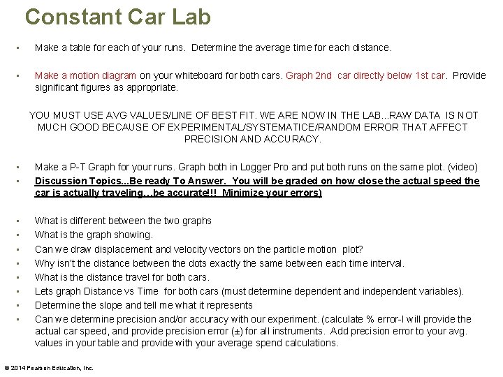
Constant Car Lab • Make a table for each of your runs. Determine the average time for each distance. • Make a motion diagram on your whiteboard for both cars. Graph 2 nd car directly below 1 st car. Provide significant figures as appropriate. YOU MUST USE AVG VALUES/LINE OF BEST FIT. WE ARE NOW IN THE LAB. . . RAW DATA IS NOT MUCH GOOD BECAUSE OF EXPERIMENTAL/SYSTEMATICE/RANDOM ERROR THAT AFFECT PRECISION AND ACCURACY. • • Make a P-T Graph for your runs. Graph both in Logger Pro and put both runs on the same plot. (video) Discussion Topics. . . Be ready To Answer. You will be graded on how close the actual speed the car is actually traveling…be accurate!!! Minimize your errors) • • What is different between the two graphs What is the graph showing. Can we draw displacement and velocity vectors on the particle motion plot? Why isn’t the distance between the dots exactly the same between each time interval. What is the distance travel for both cars. Lets graph Distance vs Time for both cars (must determine dependent and independent variables). Determine the slope and tell me what it represents Can we determine precision and/or accuracy with our experiment. (calculate % error-I will provide the actual car speed, and provide precision error (±) for all instruments. Add precision error to your avg. values in your table and provide with your average spend calculations. © 2014 Pearson Education, Inc.

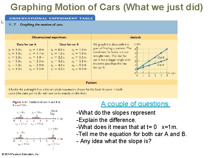
Graphing Motion of Cars (What we just did) A couple of questions. -What do the slopes represent -Explain the difference. -What does it mean that at t= 0 x=1 m. -Tell me the equation for both car A and B. - Any idea what the slope is? © 2014 Pearson Education, Inc.

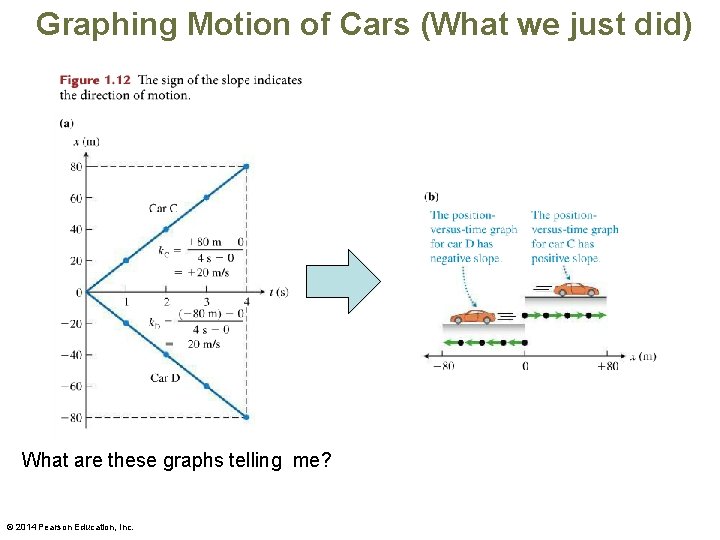
Graphing Motion of Cars (What we just did) What are these graphs telling me? © 2014 Pearson Education, Inc.

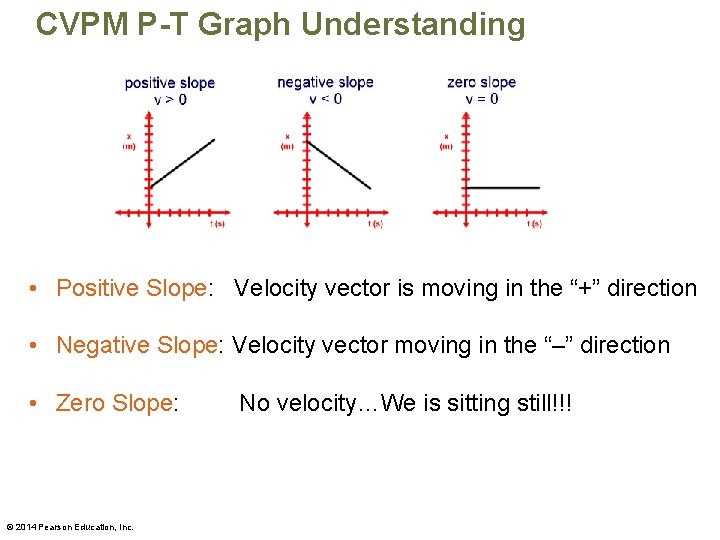
CVPM P-T Graph Understanding • Positive Slope: Velocity vector is moving in the “+” direction • Negative Slope: Velocity vector moving in the “–” direction • Zero Slope: © 2014 Pearson Education, Inc. No velocity…We is sitting still!!!

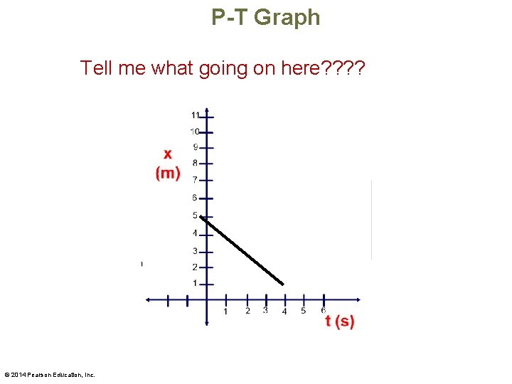
P-T Graph Tell me what going on here? ? © 2014 Pearson Education, Inc.

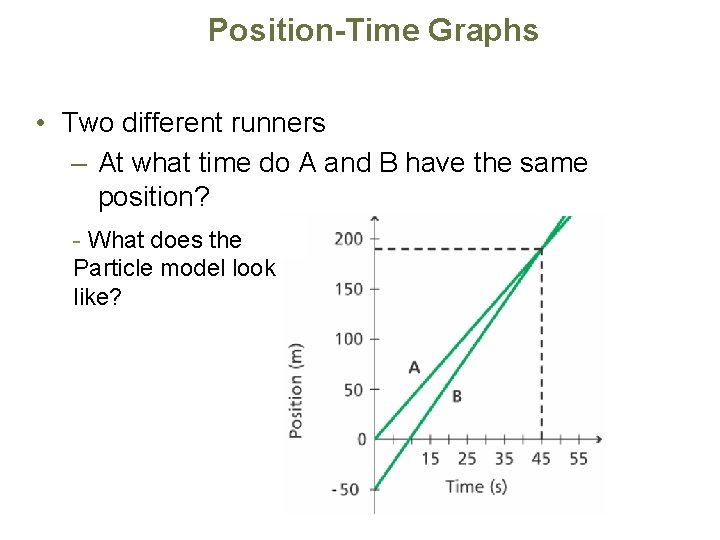
Position-Time Graphs • Two different runners – At what time do A and B have the same position? - What does the Particle model look like?

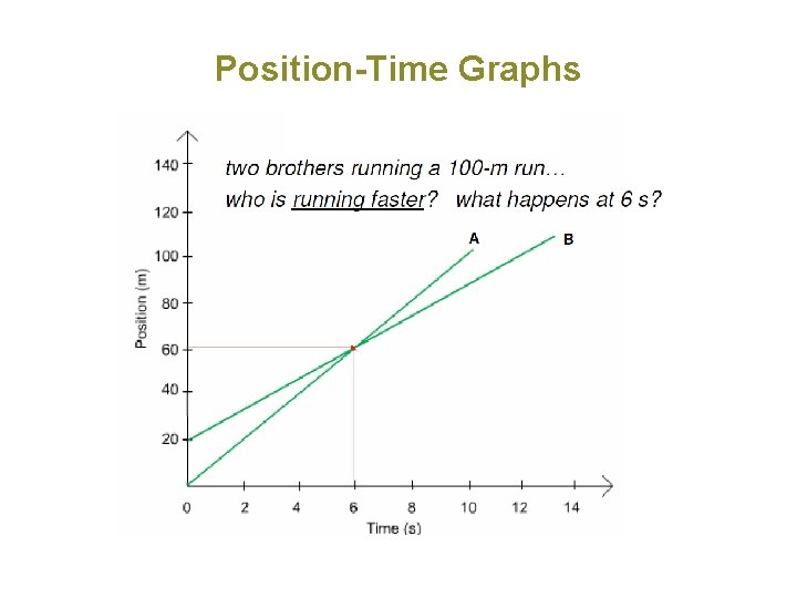
Position-Time Graphs

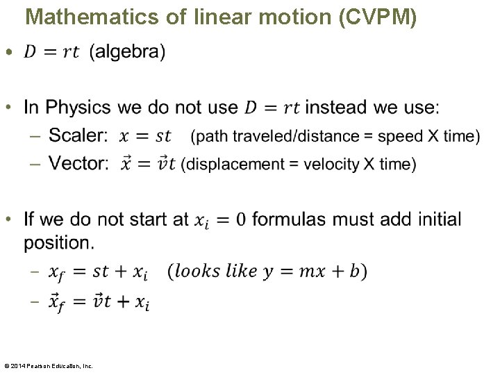
Mathematics of linear motion (CVPM) • © 2014 Pearson Education, Inc.

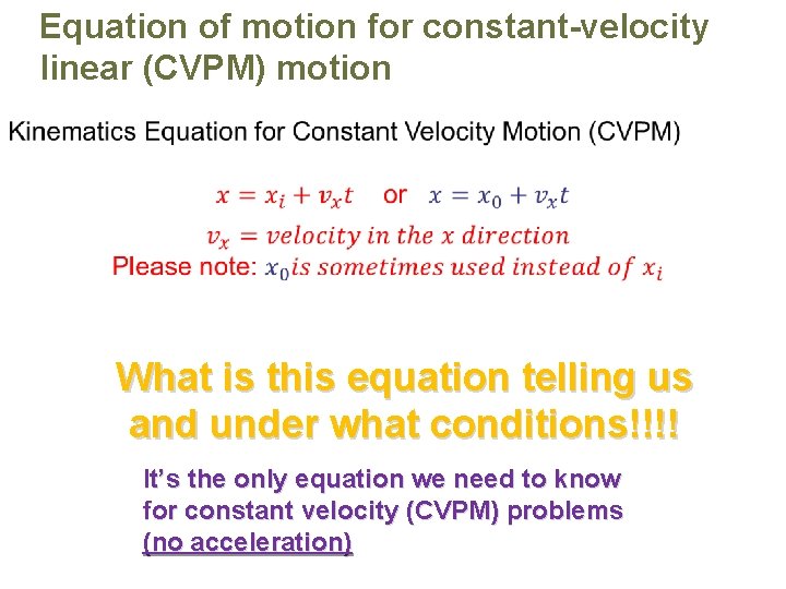
Equation of motion for constant-velocity linear (CVPM) motion What is this equation telling us and under what conditions!!!! It’s the only equation we need to know for constant velocity (CVPM) problems (no acceleration)

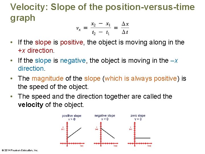
Velocity: Slope of the position-versus-time graph • If the slope is positive, the object is moving along in the +x direction. • If the slope is negative, the object is moving in the –x direction. • The magnitude of the slope (which is always positive) is the speed of the object. • The speed and the direction together are called the velocity of the object. © 2014 Pearson Education, Inc.

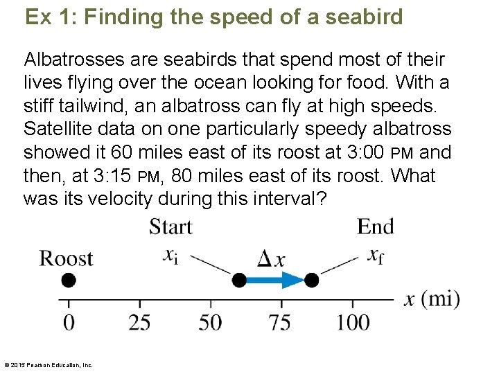
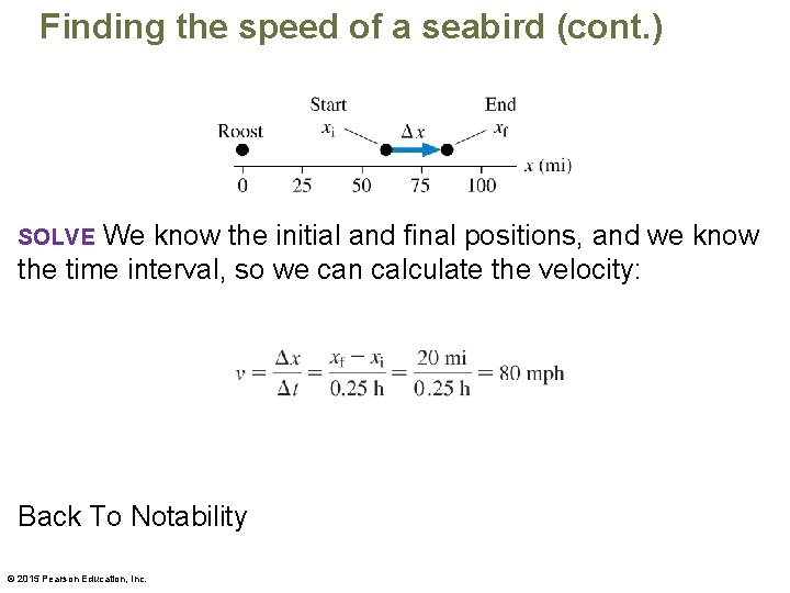
Ex 1: Finding the speed of a seabird Albatrosses are seabirds that spend most of their lives flying over the ocean looking for food. With a stiff tailwind, an albatross can fly at high speeds. Satellite data on one particularly speedy albatross showed it 60 miles east of its roost at 3: 00 PM and then, at 3: 15 PM, 80 miles east of its roost. What was its velocity during this interval? © 2015 Pearson Education, Inc.

Finding the speed of a seabird (cont. ) We know the initial and final positions, and we know the time interval, so we can calculate the velocity: SOLVE Back To Notability © 2015 Pearson Education, Inc.

The Velocity-Time Graph (V-T Graph) Graphing Velocity © 2014 Pearson Education, Inc.

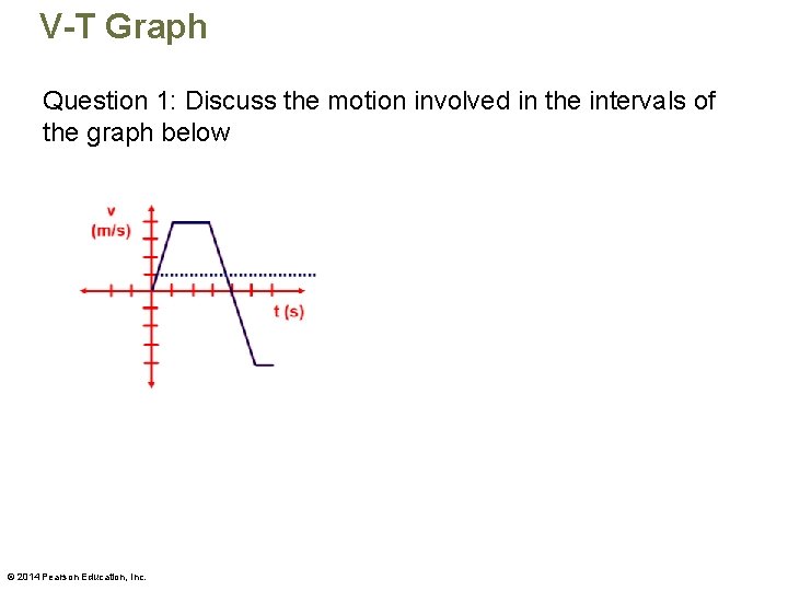
V-T Graph Question 1: Discuss the motion involved in the intervals of the graph below © 2014 Pearson Education, Inc.

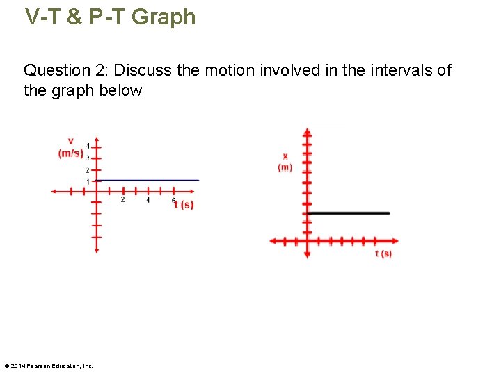
V-T & P-T Graph Question 2: Discuss the motion involved in the intervals of the graph below © 2014 Pearson Education, Inc.

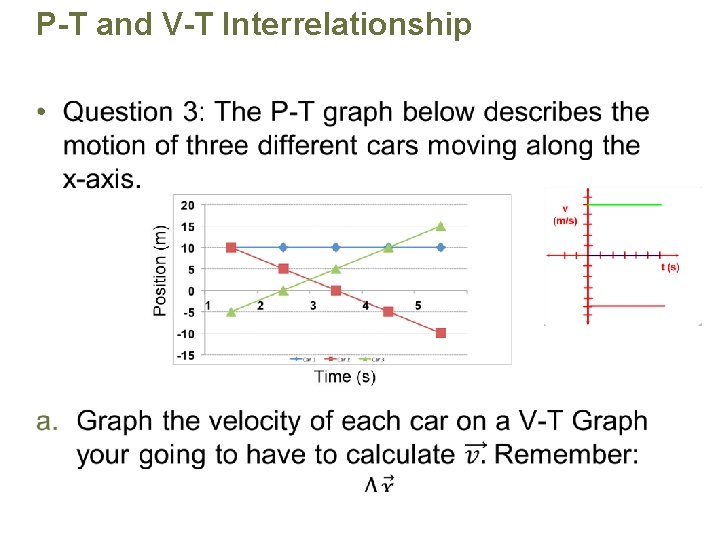
P-T and V-T Interrelationship •

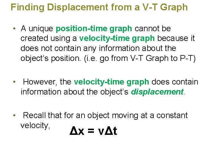
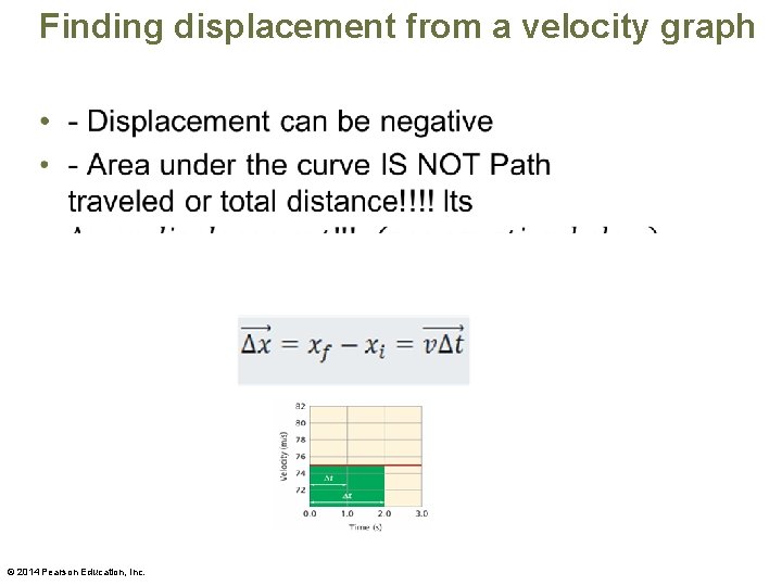
Finding Displacement from a V-T Graph • A unique position-time graph cannot be created using a velocity-time graph because it does not contain any information about the object’s position. (i. e. go from V-T Graph to P-T) • However, the velocity-time graph does contain information about the object’s displacement. • Recall that for an object moving at a constant velocity, Δx = vΔt

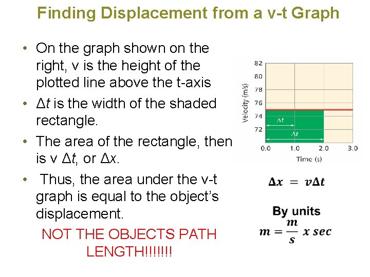
Finding Displacement from a v-t Graph • On the graph shown on the right, v is the height of the plotted line above the t-axis • Δt is the width of the shaded rectangle. • The area of the rectangle, then, is v Δt, or Δx. • Thus, the area under the v-t graph is equal to the object’s displacement. NOT THE OBJECTS PATH LENGTH!!!!!!!

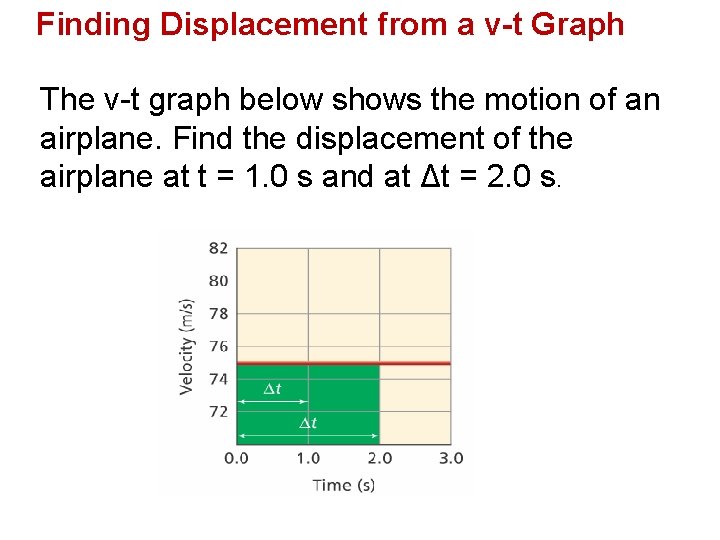
Finding Displacement from a v-t Graph The v-t graph below shows the motion of an airplane. Find the displacement of the airplane at t = 1. 0 s and at Δt = 2. 0 s.

Finding displacement from a velocity graph • © 2014 Pearson Education, Inc.

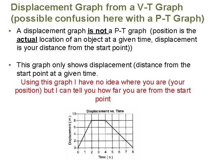
Displacement Graph from a V-T Graph (possible confusion here with a P-T Graph) • A displacement graph is not a P-T graph (position is the actual location of an object at a given time, displacement is your distance from the start point)) • This graph only shows displacement (distance from the start point at a given time. Using this graph I have no idea where you are (your position) but I can tell you how far you are from the start point

1. 6 Motion at Constant Acceleration (UAPM) © 2014 Pearson Education, Inc.

A. Acceleration Basics © 2014 Pearson Education, Inc.

Acceleration Objectives • Describe motion in terms of changing velocity. • Compare graphical representations of accelerated and nonaccelerated motions. • Apply kinematic equations to calculate distance, time, or velocity under conditions of constant acceleration.

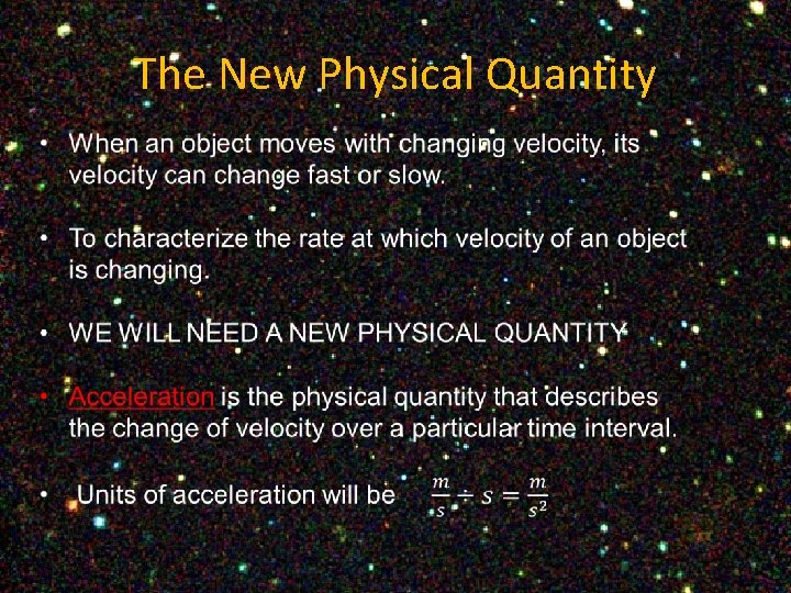
The New Physical Quantity

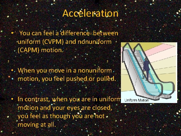
Acceleration • You can feel a difference between uniform (CVPM) and nonuniform (CAPM) motion. • When you move in a nonuniform motion, you feel pushed or pulled. • In contrast, when you are in uniform motion and your eyes are closed, you feel as though you are not moving at all.

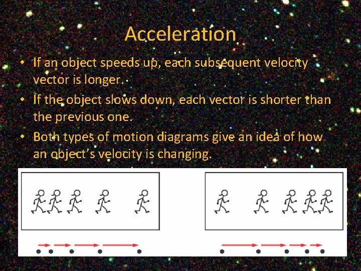
Acceleration • If an object speeds up, each subsequent velocity vector is longer. • If the object slows down, each vector is shorter than the previous one. • Both types of motion diagrams give an idea of how an object’s velocity is changing.

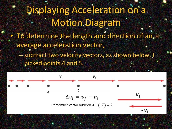
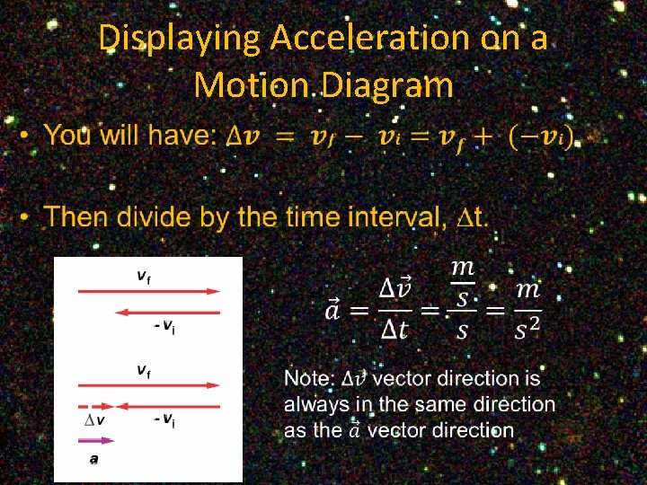
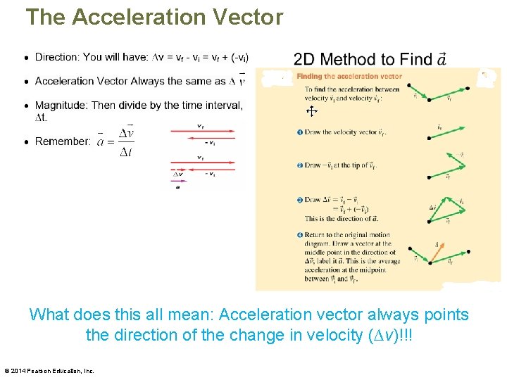
Displaying Acceleration on a Motion Diagram • To determine the length and direction of an average acceleration vector, – subtract two velocity vectors, as shown below. I picked points 4 and 5. 4 5

Displaying Acceleration on a Motion Diagram •

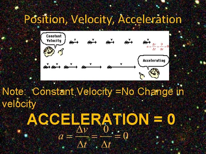
Position, Velocity, Acceleration Note: Constant Velocity =No Change in velocity ACCELERATION = 0

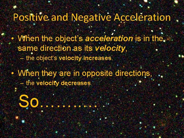
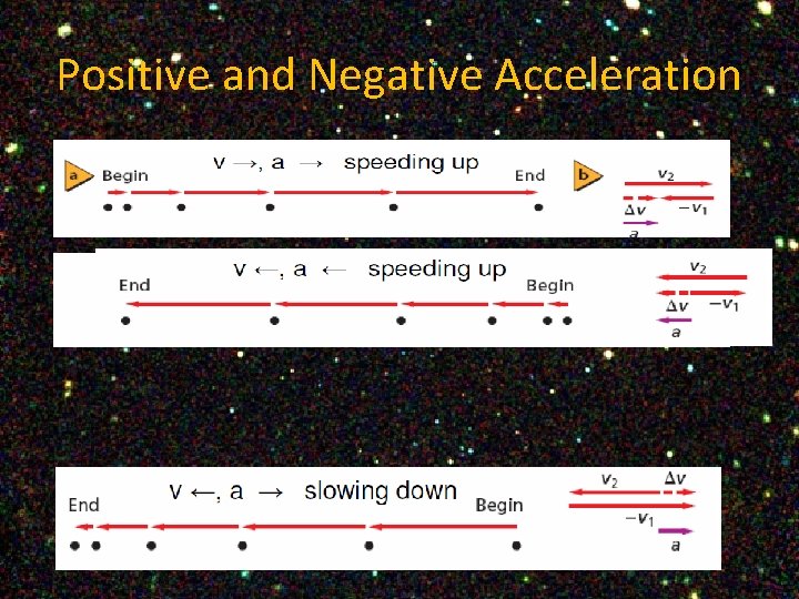
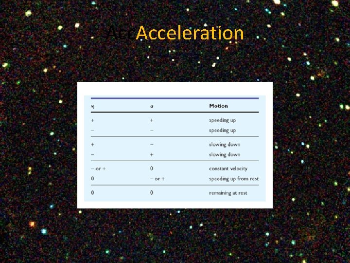
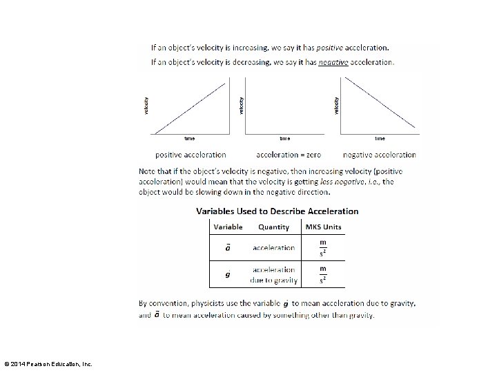
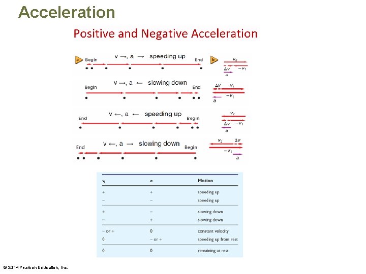
Positive and Negative Acceleration • When the object’s acceleration is in the same direction as its velocity, – the object’s velocity increases. • When they are in opposite directions, – the velocity decreases. • So……. . …

Positive and Negative Acceleration

Acc. Acceleration

Graphing Acceleration

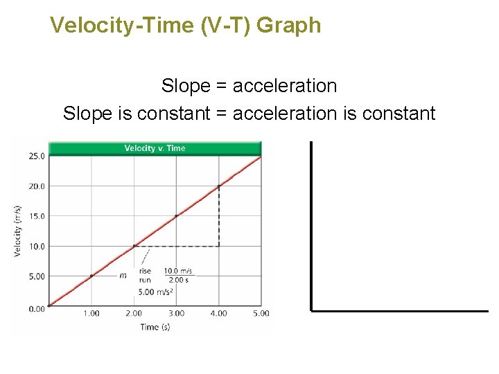
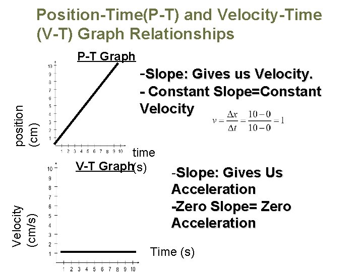
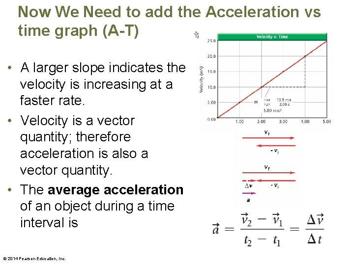
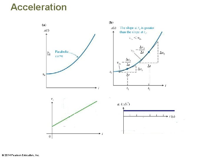
Velocity-Time (V-T) Graph Slope = acceleration Slope is constant = acceleration is constant

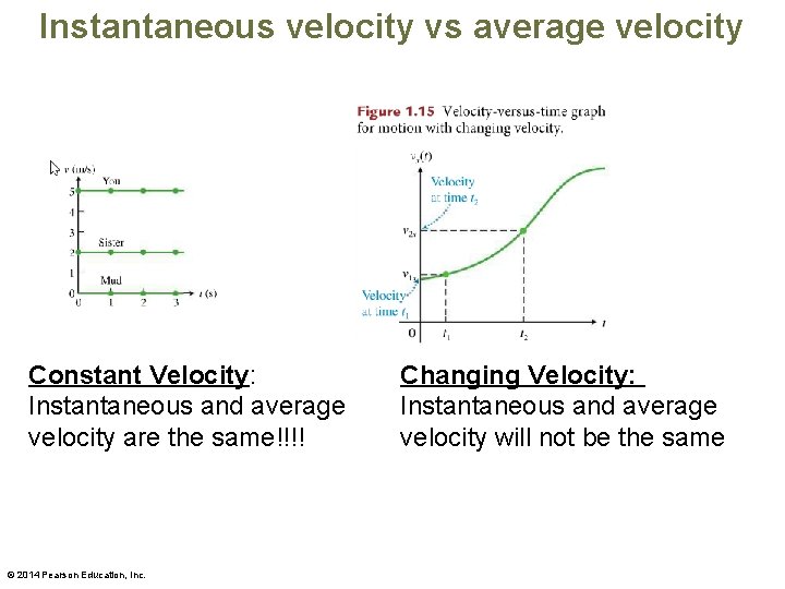
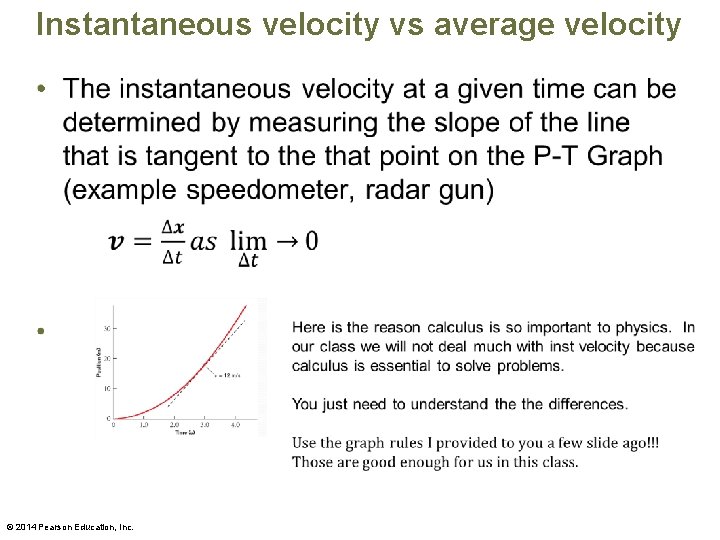
When velocity is not constant • On a V-T graph, velocity will be a straight line only if it is a constant (not changing!!). However, velocity will not be constant all the time…. • Two Types of velocity we use in physics: – Instantaneous velocity is the velocity of an object at a particular time. – Average velocity is the ratio of the change in position and the time interval during which this change occurred. – Note: For motion at constant velocity, the instantaneous and average velocities are equal; for motion with changing velocity, they are not. © 2014 Pearson Education, Inc.

Instantaneous velocity vs average velocity Constant Velocity: Instantaneous and average velocity are the same!!!! © 2014 Pearson Education, Inc. Changing Velocity: Instantaneous and average velocity will not be the same

Instantaneous velocity vs average velocity • © 2014 Pearson Education, Inc.

Position-Time(P-T) and Velocity-Time (V-T) Graph Relationships P-T Graph Velocity (cm/s) position (cm) -Slope: Gives us Velocity. - Constant Slope=Constant Velocity time V-T Graph(s) -Slope: Gives Us Acceleration -Zero Slope= Zero Acceleration Time (s)

Now We Need to add the Acceleration vs time graph (A-T) • A larger slope indicates the velocity is increasing at a faster rate. • Velocity is a vector quantity; therefore acceleration is also a vector quantity. • The average acceleration of an object during a time interval is © 2014 Pearson Education, Inc.

© 2014 Pearson Education, Inc.

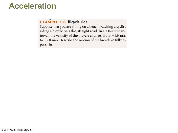
Acceleration © 2014 Pearson Education, Inc.

The Acceleration Vector What does this all mean: Acceleration vector always points the direction of the change in velocity (∆v)!!! © 2014 Pearson Education, Inc.

Kinematic Equations © 2014 Pearson Education, Inc.

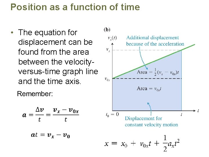
Position as a function of time • The equation for displacement can be found from the area between the velocityversus-time graph line and the time axis.

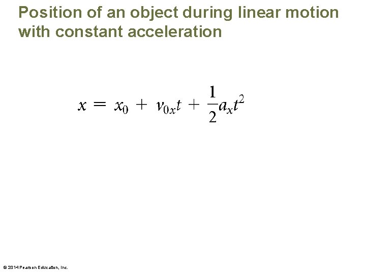
Position of an object during linear motion with constant acceleration © 2014 Pearson Education, Inc.

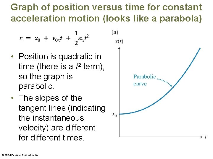
Graph of position versus time for constant acceleration motion (looks like a parabola) • Position is quadratic in time (there is a t 2 term), so the graph is parabolic. • The slopes of the tangent lines (indicating the instantaneous velocity) are different for different times. © 2014 Pearson Education, Inc.

Acceleration © 2014 Pearson Education, Inc.

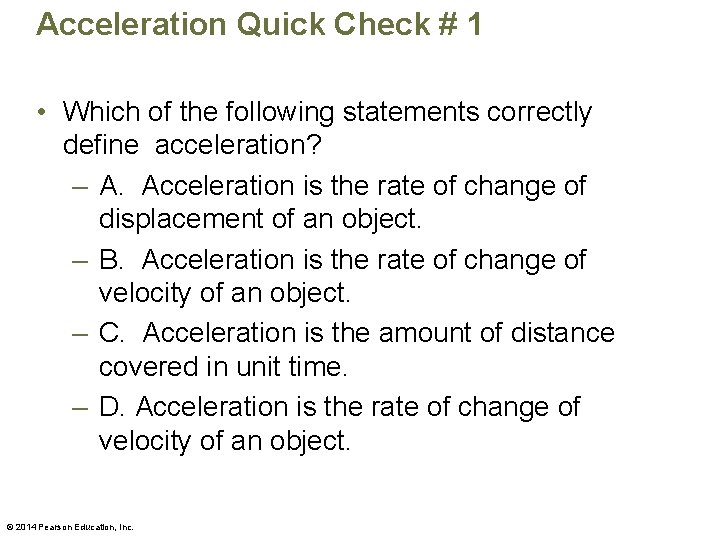
Acceleration Quick Check # 1 • Which of the following statements correctly define acceleration? – A. Acceleration is the rate of change of displacement of an object. – B. Acceleration is the rate of change of velocity of an object. – C. Acceleration is the amount of distance covered in unit time. – D. Acceleration is the rate of change of velocity of an object. © 2014 Pearson Education, Inc.

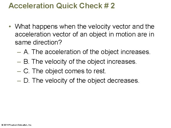
Acceleration Quick Check # 2 • What happens when the velocity vector and the acceleration vector of an object in motion are in same direction? – A. The acceleration of the object increases. – B. The velocity of the object increases. – C. The object comes to rest. – D. The velocity of the object decreases. © 2014 Pearson Education, Inc.

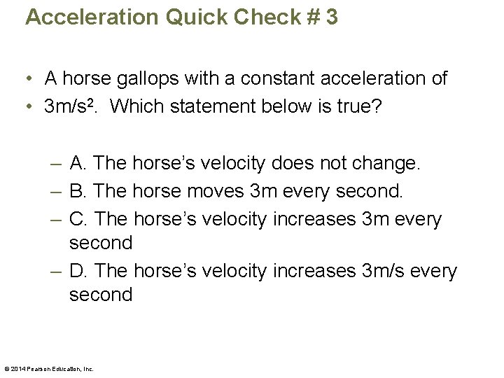
Acceleration Quick Check # 3 • A horse gallops with a constant acceleration of • 3 m/s 2. Which statement below is true? – A. The horse’s velocity does not change. – B. The horse moves 3 m every second. – C. The horse’s velocity increases 3 m every second – D. The horse’s velocity increases 3 m/s every second © 2014 Pearson Education, Inc.

Acceleration © 2014 Pearson Education, Inc.

Acceleration © 2014 Pearson Education, Inc.

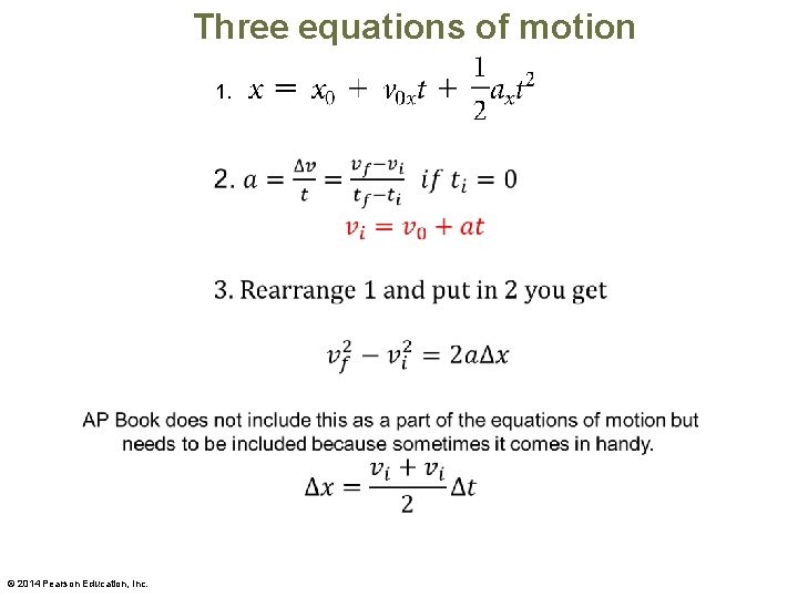
Three equations of motion 1. © 2014 Pearson Education, Inc.

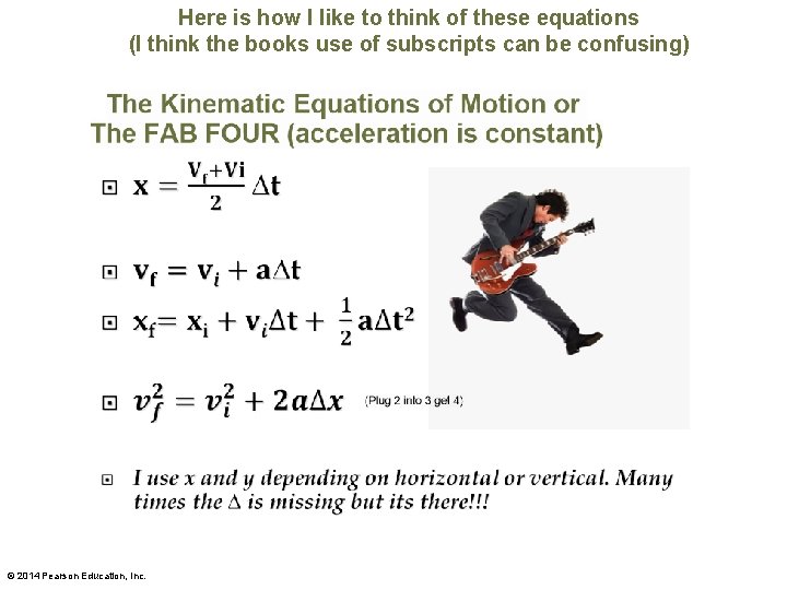
Here is how I like to think of these equations (I think the books use of subscripts can be confusing) © 2014 Pearson Education, Inc.

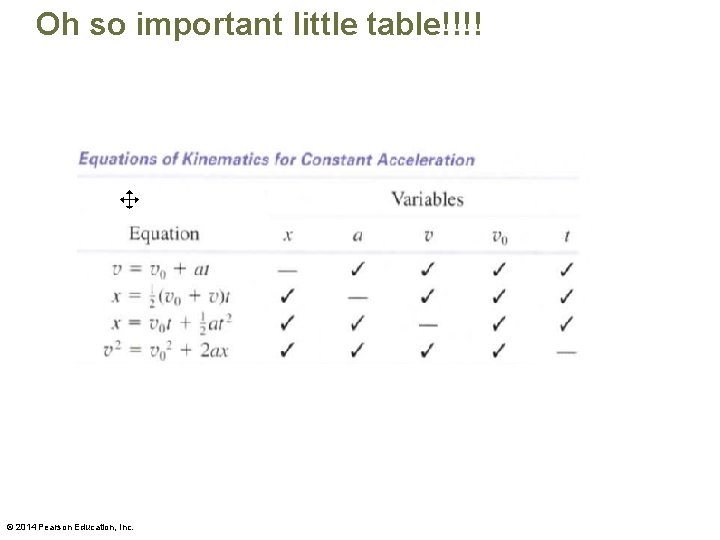
Oh so important little table!!!! © 2014 Pearson Education, Inc.

1. 7 Skills for analyzing situations involving motion © 2014 Pearson Education, Inc.

Skills for analyzing situations involving motion • Represent processes in multiple ways: – The words in the problem statement – A sketch – One or more diagrams – Possibly a graph – A mathematical description • Different representations have to agree with each other; they need to be consistent. © 2014 Pearson Education, Inc.

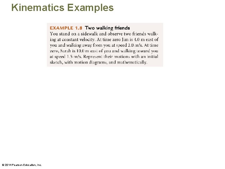
Kinematics Examples © 2014 Pearson Education, Inc.

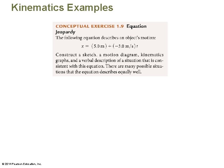
Kinematics Examples © 2014 Pearson Education, Inc.

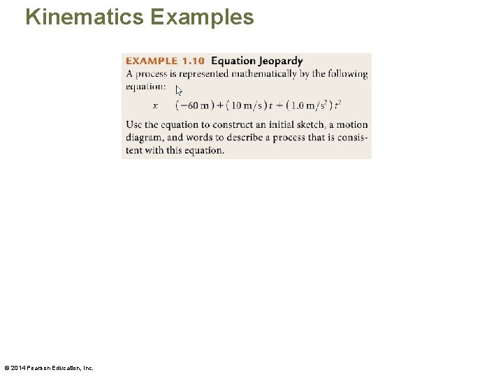
Kinematics Examples © 2014 Pearson Education, Inc.

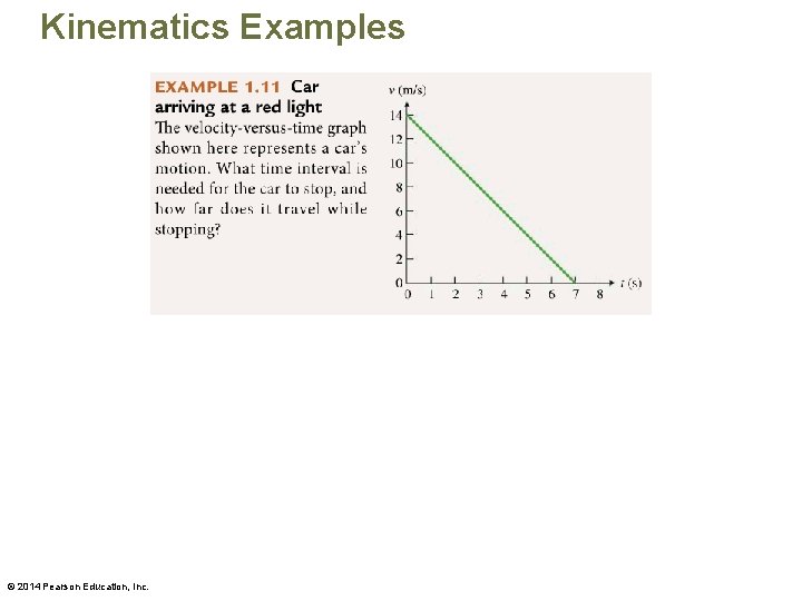
Kinematics Examples © 2014 Pearson Education, Inc.

1. 8 Free Fall © 2014 Pearson Education, Inc.

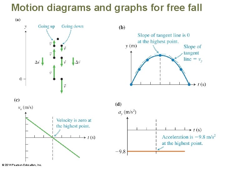
Free Fall • In this chapter we learned about 2 simple models of motion – Linear motion (1 D)with constant velocity – Linear motion (1 D) with constant acceleration (fab 4) – Now we will talk about a special case of linear motion----- the motion of falling objects – Ball Drop demo and the moon video!!! © 2014 Pearson Education, Inc.

Free Fall and Mr. Galileo • Galileo concluded: – neglecting the effect of the air, all objects in free fall had the same acceleration. – It didn’t matter what they were made of, how much they weighed, what height they were dropped from, or whether they were dropped or thrown. – The acceleration of falling objects, given a special symbol, g, is equal to 9. 80 m/s 2. We can use 10 m/s 2 in most of our calculations. – The acceleration due to gravity is the acceleration of an object in free fall. © 2014 Pearson Education, Inc.

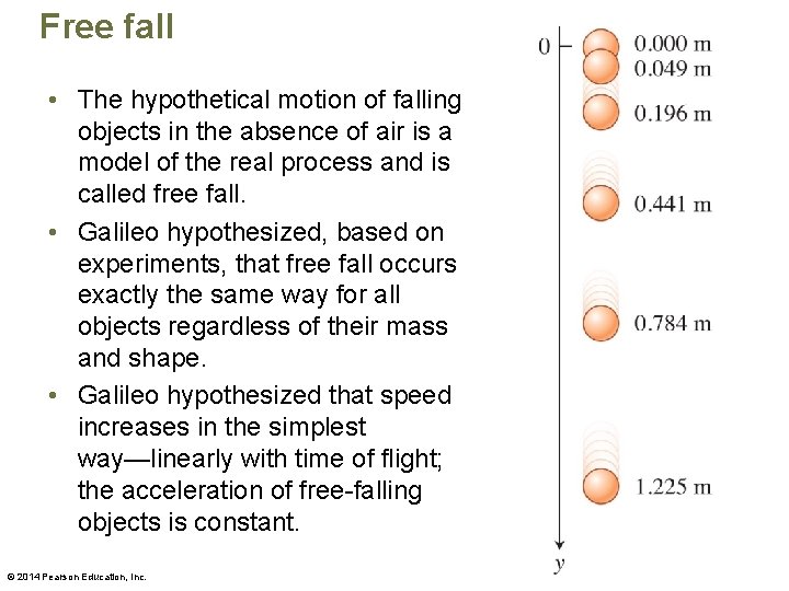
Free fall • The hypothetical motion of falling objects in the absence of air is a model of the real process and is called free fall. • Galileo hypothesized, based on experiments, that free fall occurs exactly the same way for all objects regardless of their mass and shape. • Galileo hypothesized that speed increases in the simplest way—linearly with time of flight; the acceleration of free-falling objects is constant. © 2014 Pearson Education, Inc.

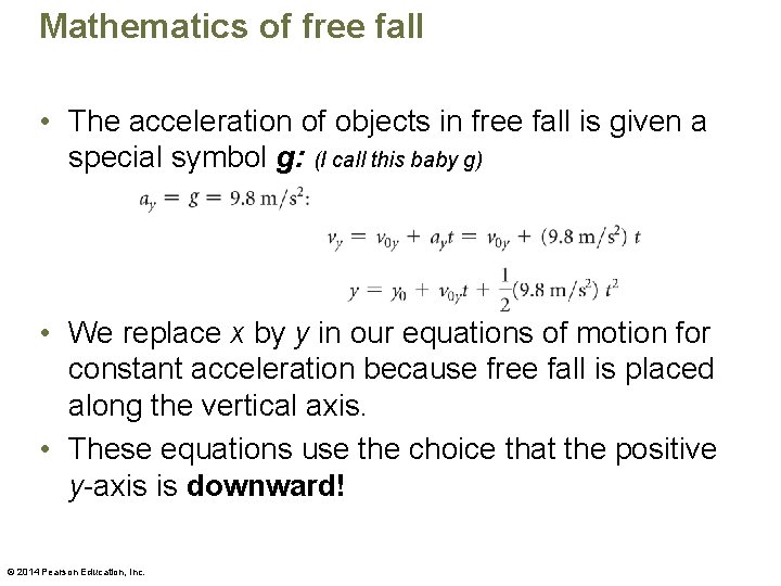
Mathematics of free fall • The acceleration of objects in free fall is given a special symbol g: (I call this baby g) • We replace x by y in our equations of motion for constant acceleration because free fall is placed along the vertical axis. • These equations use the choice that the positive y-axis is downward! © 2014 Pearson Education, Inc.

Motion diagrams and graphs for free fall © 2014 Pearson Education, Inc.

Free Fall Quick Questions • If everything accelerates at the same rate, does that means everything fall at the same rate (neglect air resistance)? • Even if they have a different weight? • Even if they are different sizes and shape? © 2014 Pearson Education, Inc.

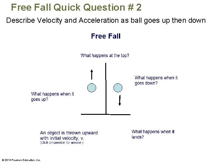
Free Fall Quick Question # 2 Describe Velocity and Acceleration as ball goes up then down © 2014 Pearson Education, Inc.

Free Fall Quick Question # 3 • A ball is tossed straight up in the air. At its very highest point, the balls instantaneous acceleration ay is • A. Positive • B. Negative • C. zero © 2014 Pearson Education, Inc.

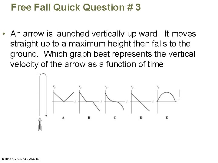
Free Fall Quick Question # 3 • An arrow is launched vertically up ward. It moves straight up to a maximum height then falls to the ground. Which graph best represents the vertical velocity of the arrow as a function of time t © 2014 Pearson Education, Inc.

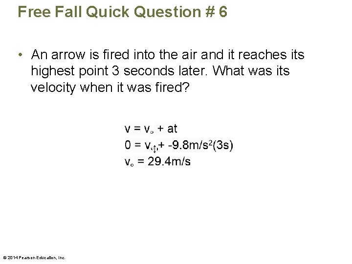
Free Fall Quick Question # 6 • An arrow is fired into the air and it reaches its highest point 3 seconds later. What was its velocity when it was fired? © 2014 Pearson Education, Inc.

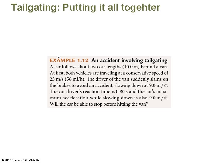
Tailgating: Putting it all togehter © 2014 Pearson Education, Inc.