Automatic Panoramic Image Stitching using Local Features Matthew

Automatic Panoramic Image Stitching using Local Features Matthew Brown and David Lowe, University of British Columbia

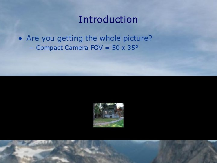
Introduction • Are you getting the whole picture? – Compact Camera FOV = 50 x 35°

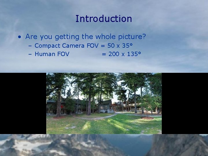
Introduction • Are you getting the whole picture? – Compact Camera FOV = 50 x 35° – Human FOV = 200 x 135°

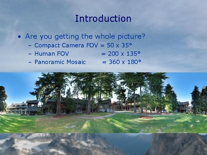
Introduction • Are you getting the whole picture? – Compact Camera FOV = 50 x 35° – Human FOV = 200 x 135° – Panoramic Mosaic = 360 x 180°

Why Use Local Features?

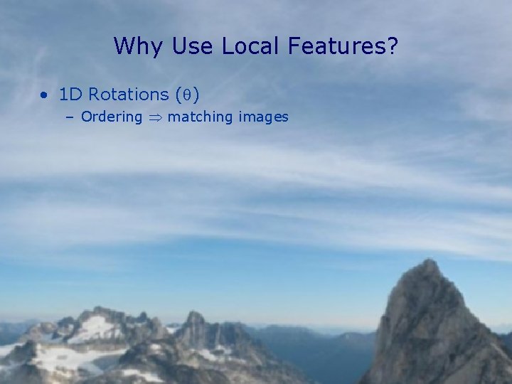
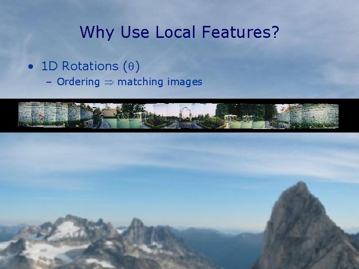
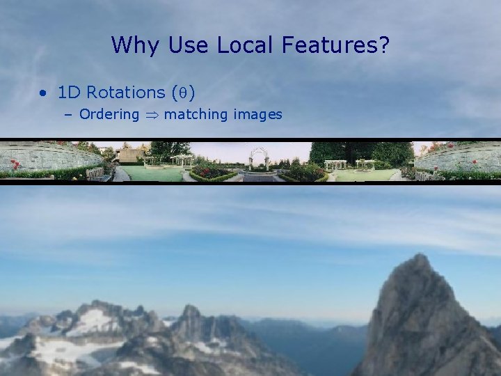
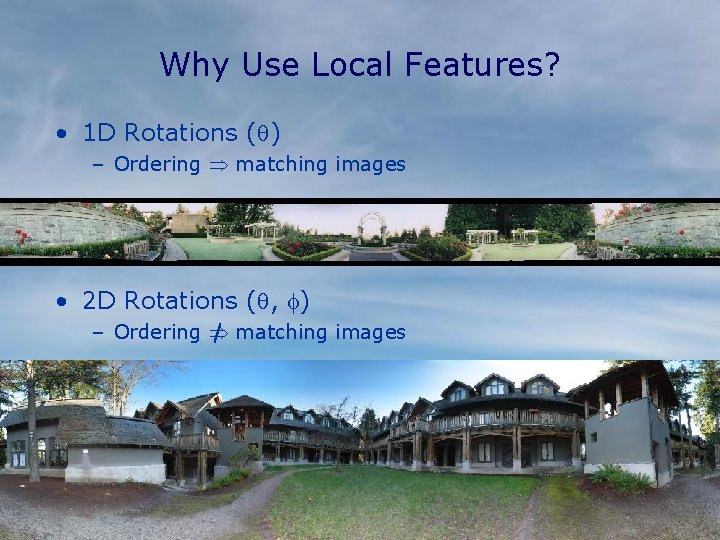
Why Use Local Features? • 1 D Rotations (q) – Ordering matching images

Why Use Local Features? • 1 D Rotations (q) – Ordering matching images

Why Use Local Features? • 1 D Rotations (q) – Ordering matching images

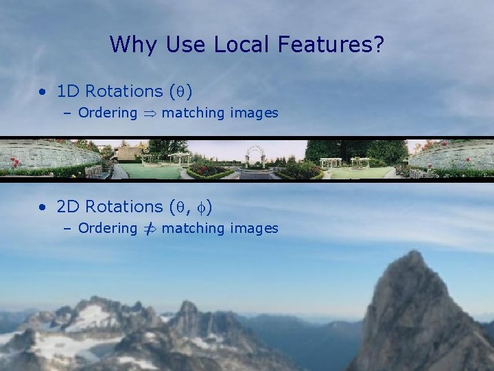
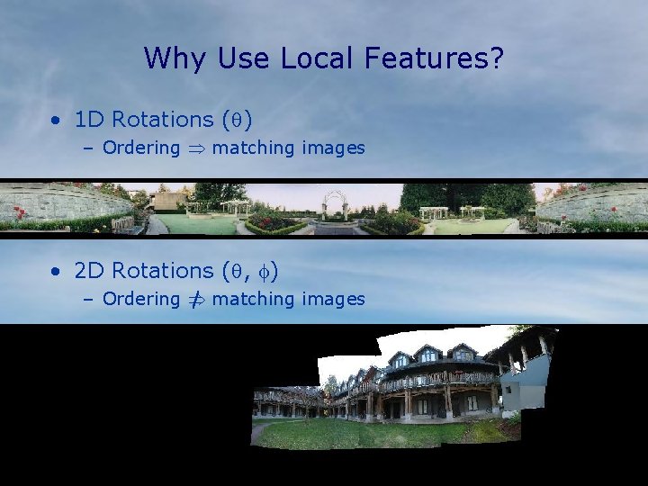
Why Use Local Features? • 1 D Rotations (q) – Ordering matching images • 2 D Rotations (q, f) – Ordering matching images

Why Use Local Features? • 1 D Rotations (q) – Ordering matching images • 2 D Rotations (q, f) – Ordering matching images

Why Use Local Features? • 1 D Rotations (q) – Ordering matching images • 2 D Rotations (q, f) – Ordering matching images

Recognising Panoramas [ Brown and Lowe ICCV 2003, IJCV 2007 ]

Automatic Stitching • • • Feature Matching Image Alignment Rendering Results Conclusions

Automatic Stitching • Feature Matching – SIFT Features – Nearest Neighbour Matching • • • Image Matching Image Alignment Rendering Results Conclusions

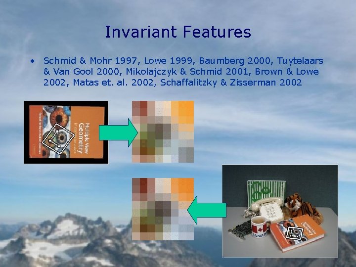
Invariant Features • Schmid & Mohr 1997, Lowe 1999, Baumberg 2000, Tuytelaars & Van Gool 2000, Mikolajczyk & Schmid 2001, Brown & Lowe 2002, Matas et. al. 2002, Schaffalitzky & Zisserman 2002

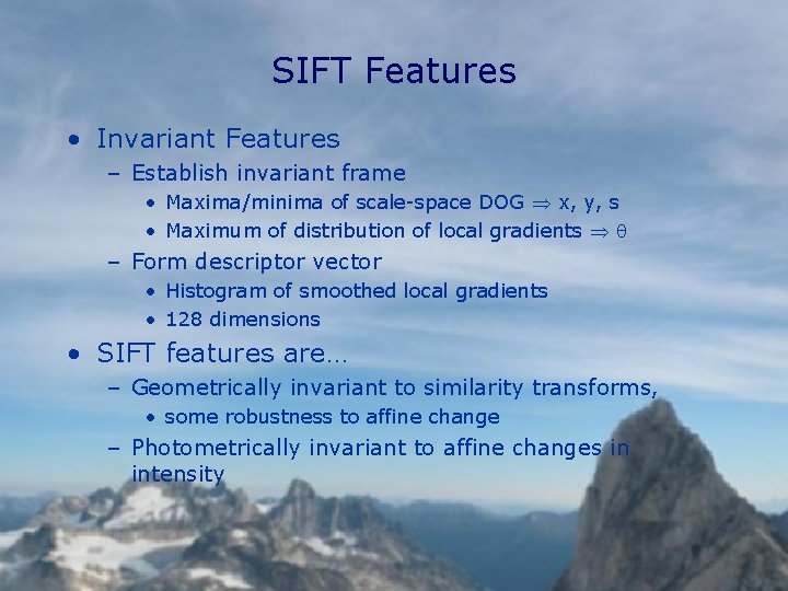
SIFT Features • Invariant Features – Establish invariant frame • Maxima/minima of scale-space DOG x, y, s • Maximum of distribution of local gradients q – Form descriptor vector • Histogram of smoothed local gradients • 128 dimensions • SIFT features are… – Geometrically invariant to similarity transforms, • some robustness to affine change – Photometrically invariant to affine changes in intensity

Automatic Stitching • Feature Matching – SIFT Features – Nearest Neighbour Matching • • • Image Matching Image Alignment Rendering Results Conclusions

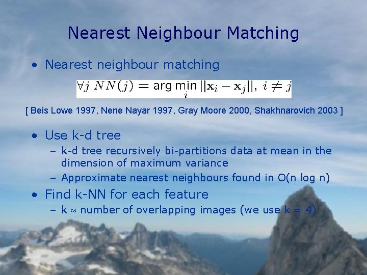
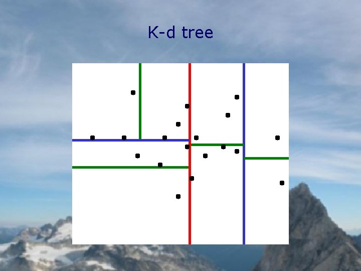
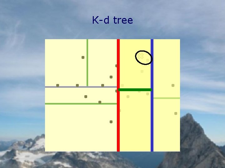
Nearest Neighbour Matching • Nearest neighbour matching [ Beis Lowe 1997, Nene Nayar 1997, Gray Moore 2000, Shakhnarovich 2003 ] • Use k-d tree – k-d tree recursively bi-partitions data at mean in the dimension of maximum variance – Approximate nearest neighbours found in O(n log n) • Find k-NN for each feature – k number of overlapping images (we use k = 4)

K-d tree

K-d tree

Automatic Stitching • Feature Matching • Image Matching – Motion Model – RANSAC • • Image Alignment Rendering Results Conclusions

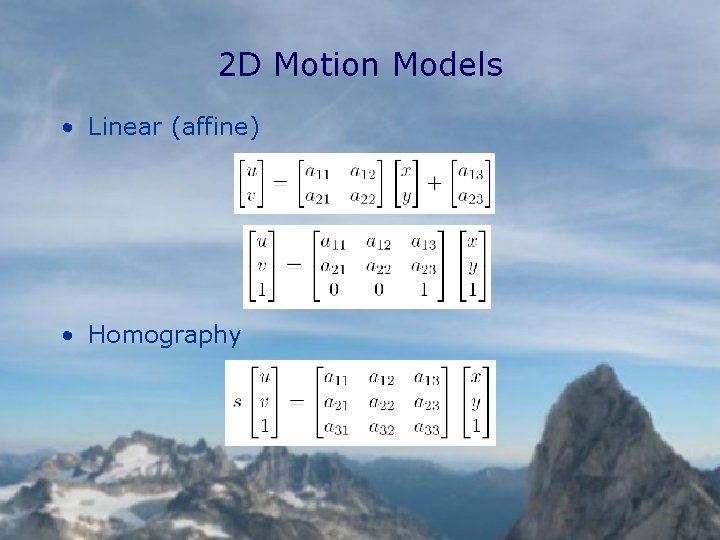
2 D Motion Models • Linear (affine) • Homography

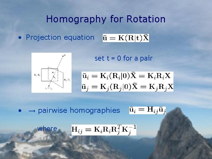
Homography for Rotation • Projection equation set t = 0 for a pair • → pairwise homographies where

Automatic Stitching • Feature Matching • Image Matching – Motion Model – RANSAC • • Image Alignment Rendering Results Conclusions

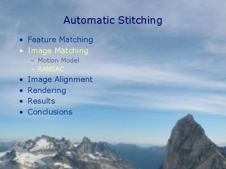
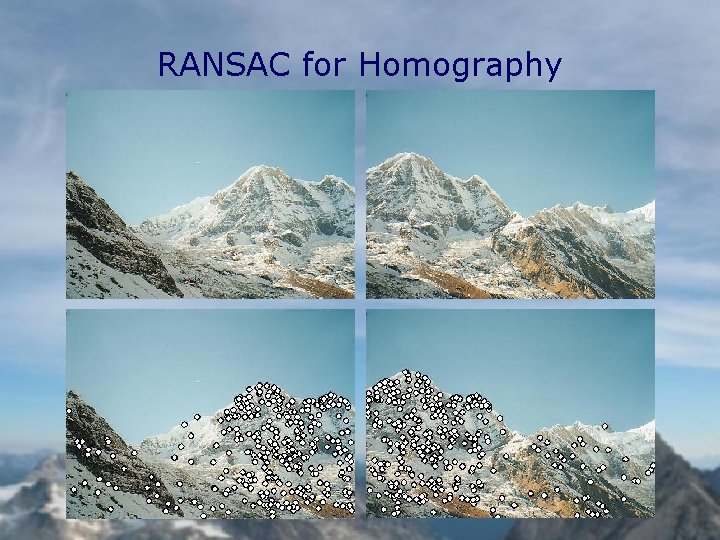
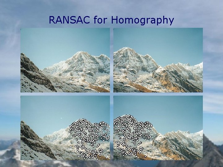
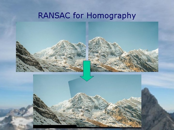
RANSAC for Homography

RANSAC for Homography

RANSAC for Homography

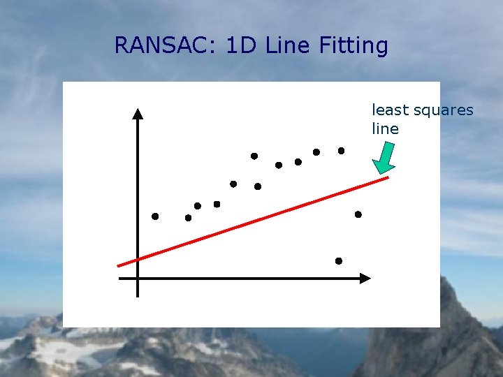
RANSAC: 1 D Line Fitting least squares line

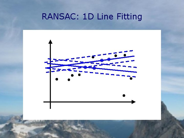
RANSAC: 1 D Line Fitting

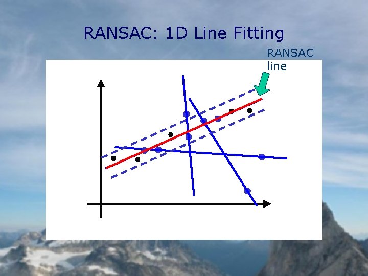
RANSAC: 1 D Line Fitting RANSAC line

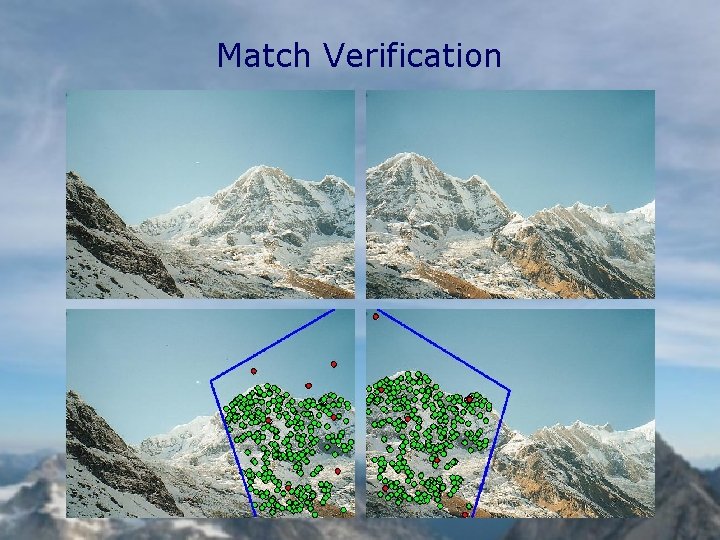
Match Verification

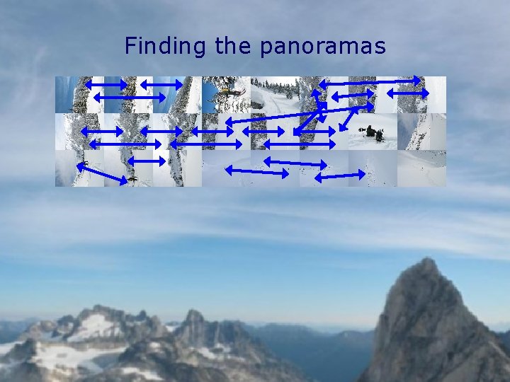
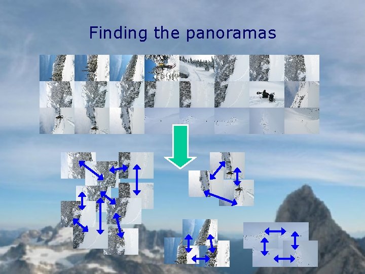
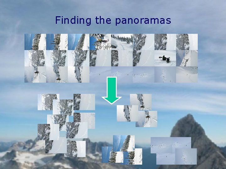
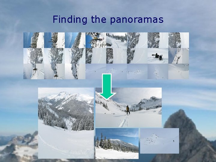
Finding the panoramas

Finding the panoramas

Finding the panoramas

Finding the panoramas

Automatic Stitching • Feature Matching • Image Alignment – Bundle Adjustment – Automatic Straightening • Rendering • Results • Conclusions

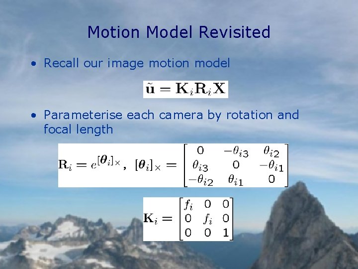
Motion Model Revisited • Recall our image motion model • Parameterise each camera by rotation and focal length

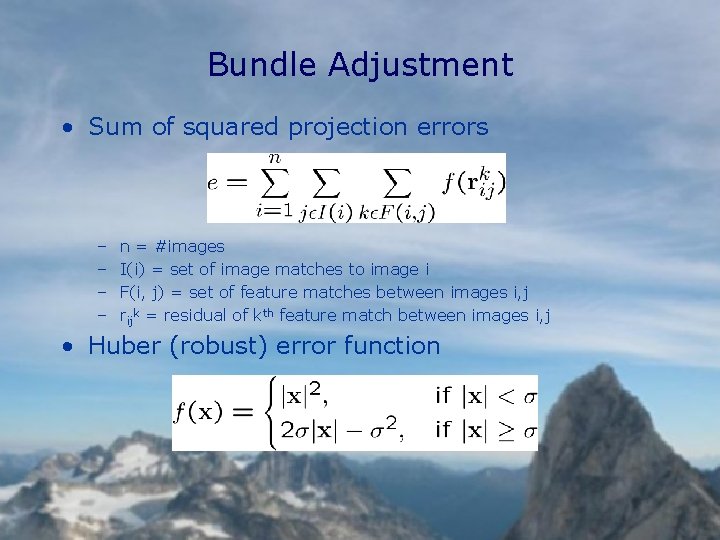
Bundle Adjustment • Sum of squared projection errors – – n = #images I(i) = set of image matches to image i F(i, j) = set of feature matches between images i, j rijk = residual of kth feature match between images i, j • Huber (robust) error function

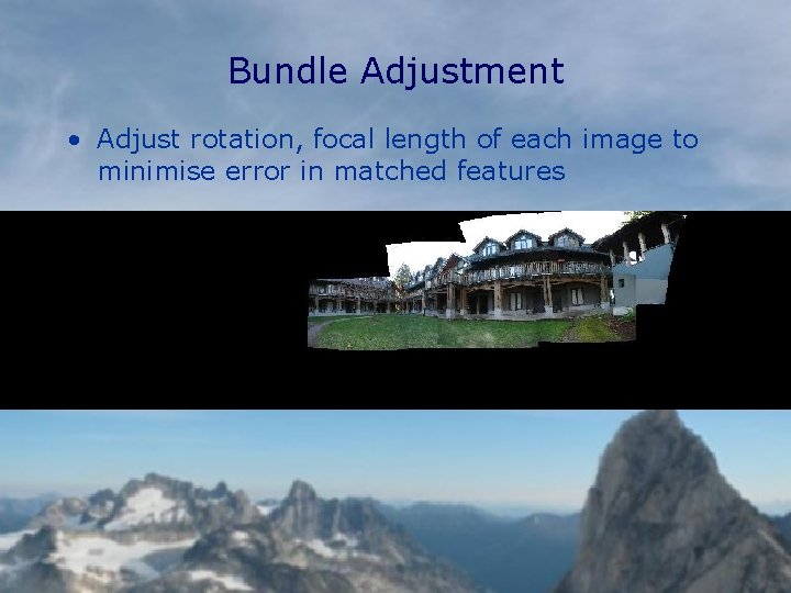
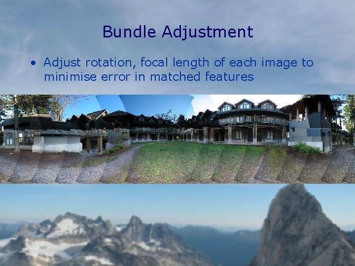
Bundle Adjustment • Adjust rotation, focal length of each image to minimise error in matched features

Bundle Adjustment • Adjust rotation, focal length of each image to minimise error in matched features

Automatic Stitching • Feature Matching • Image Alignment – Bundle Adjustment – Automatic Straightening • Rendering • Results • Conclusions

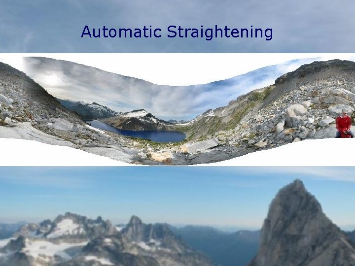
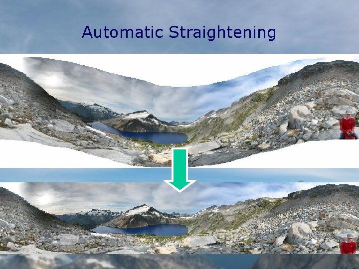
Automatic Straightening

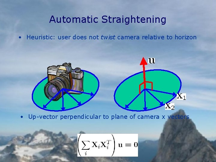
Automatic Straightening • Heuristic: user does not twist camera relative to horizon • Up-vector perpendicular to plane of camera x vectors

Automatic Straightening

Automatic Stitching • • • Feature Matching Image Alignment Rendering Results Conclusions

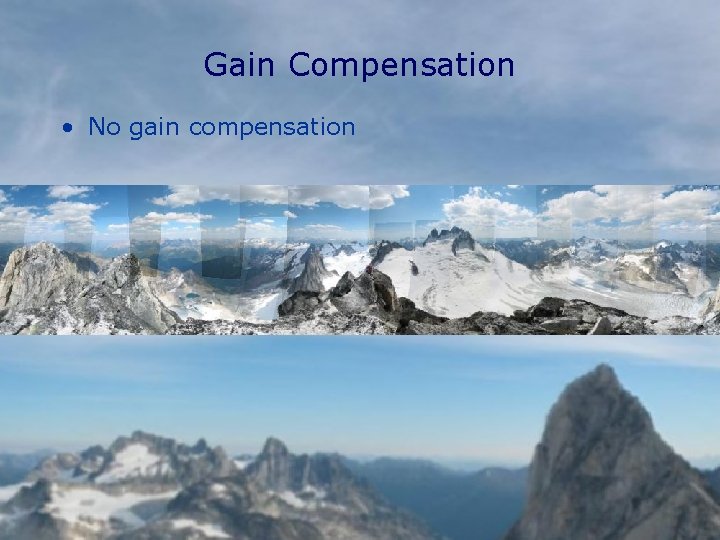
Gain Compensation • No gain compensation

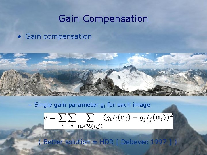
Gain Compensation • Gain compensation – Single gain parameter gi for each image ( Better solution = HDR [ Debevec 1997 ] )

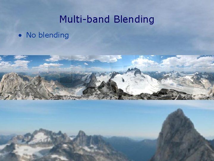
Multi-band Blending • No blending

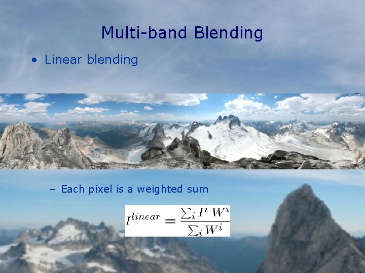
Multi-band Blending • Linear blending – Each pixel is a weighted sum

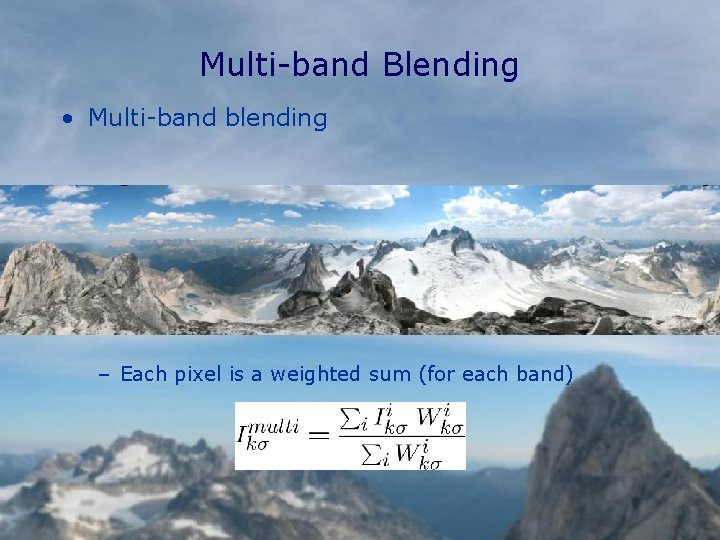
Multi-band Blending • Multi-band blending – Each pixel is a weighted sum (for each band)

Multi-band Blending • Linear blending • Multi-band blending [ Burt Adelson 1983 ]

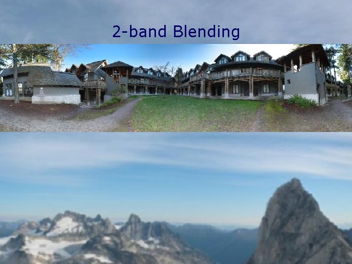
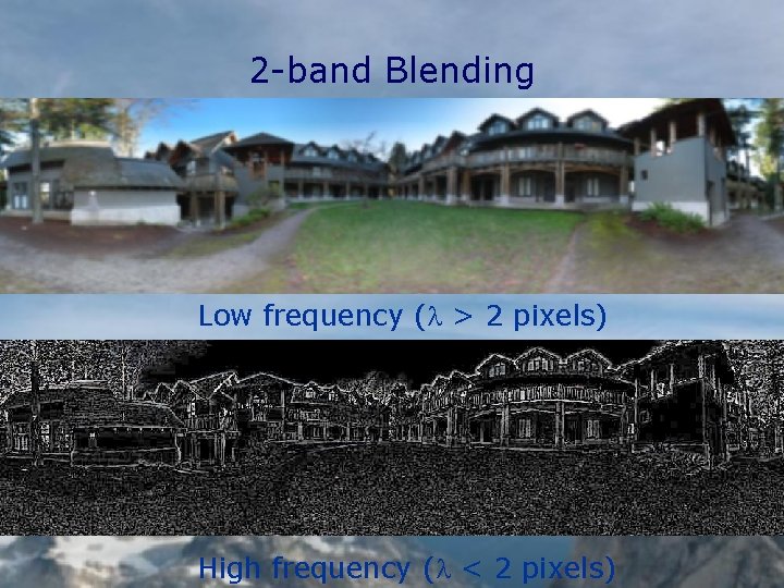
2 -band Blending

2 -band Blending Low frequency (l > 2 pixels) High frequency (l < 2 pixels)

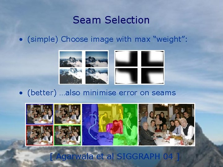
Seam Selection • (simple) Choose image with max “weight”: • (better) …also minimise error on seams [ Agarwala et al SIGGRAPH 04 ]

Automatic Stitching • • • Feature Matching Image Alignment Rendering Results Conclusions

Demo

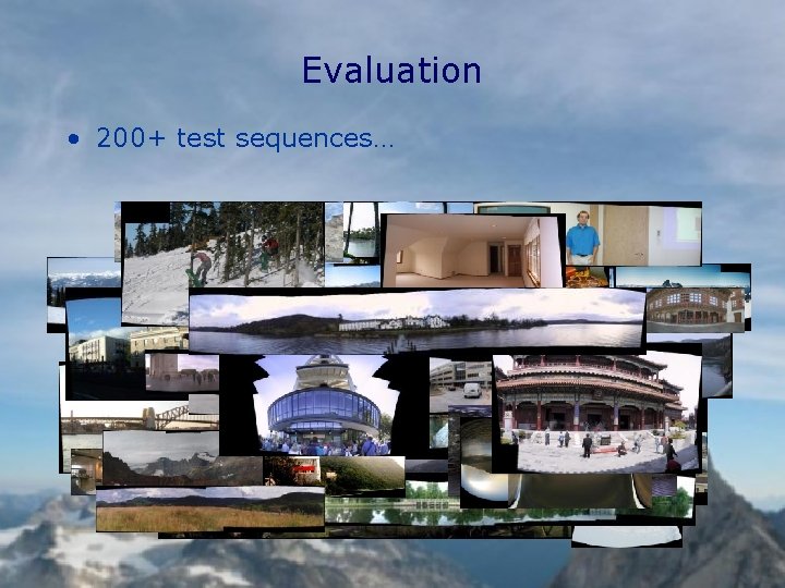
Evaluation • 200+ test sequences…

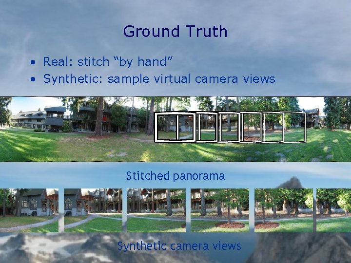
Ground Truth • Real: stitch “by hand” • Synthetic: sample virtual camera views Stitched panorama Synthetic camera views

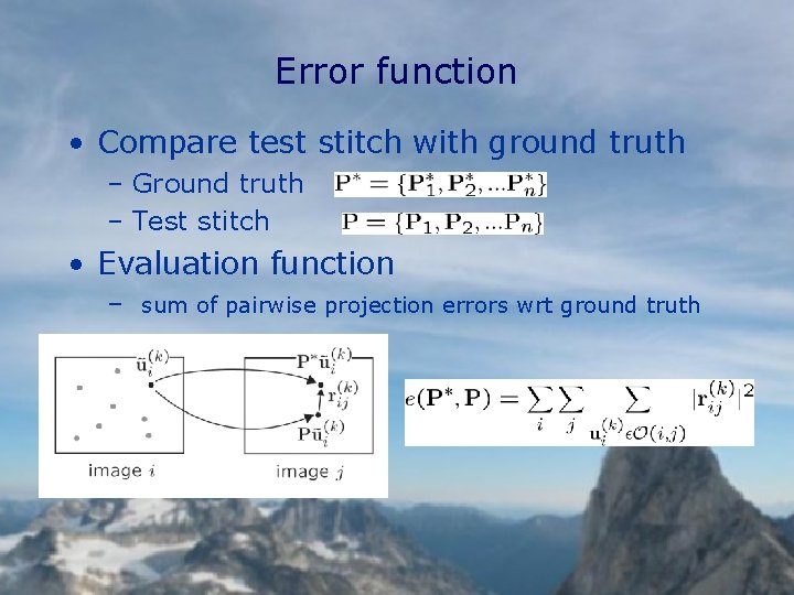
Error function • Compare test stitch with ground truth – Ground truth – Test stitch • Evaluation function – sum of pairwise projection errors wrt ground truth

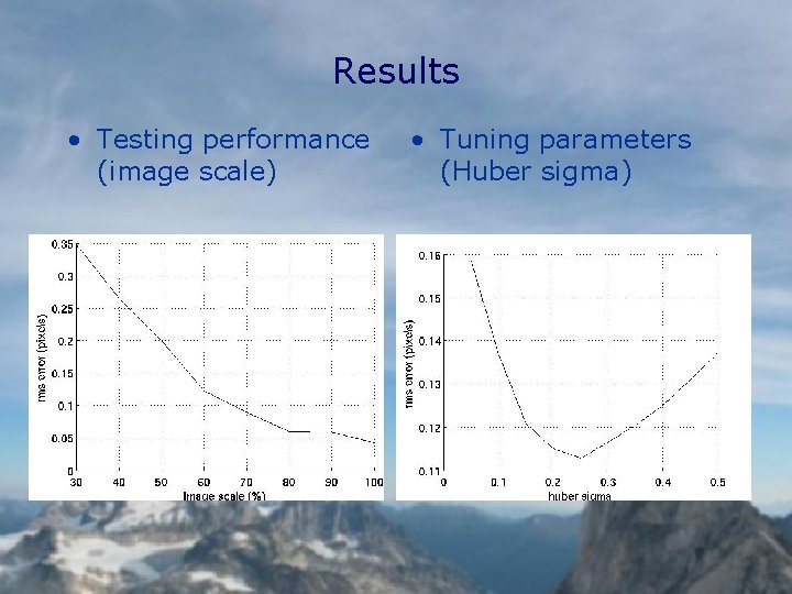
Results • Testing performance (image scale) • Tuning parameters (Huber sigma)

Conclusions • Image Stitching using Local Features – c. f. “direct methods”: fast, robust, – 2 D stitching is a recognition problem • Multi-Image Matching Framework – Local features, RANSAC, bundle adjustment, blending • Future Work – camera model += radial distortion, camera translation, scene motion, vignetting, HDR, flash … – Full 3 D case • e. g. Photo Tourism [Snavely et al SIGGRAPH 2006] http: //research. microsoft. com/~brown