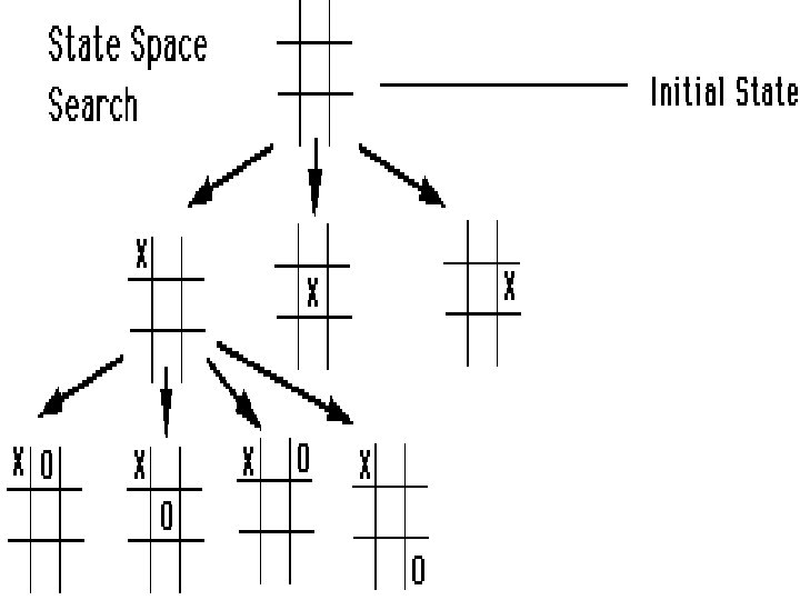
Artificial Intelligence Search Problem 2 Uninformed and informed

Artificial Intelligence Search Problem (2)

Uninformed and informed searches Breadth-first search Since we know what the goal state is like, is it possible get there faster? Oracle path

Heuristic Search Heuristics means choosing branches in a state space (when no exact solution available as in medical diagnostic or computational cost very high as in chess) that are most likely to be acceptable problem solution.

Informed search • So far, have assumed that no nongoal state looks better than another • Unrealistic – Even without knowing the road structure, some locations seem closer to the goal than others – Some states of the 8 s puzzle seem closer to the goal than others • Makes sense to expand closer-seeming nodes first

Heuristic Merriam-Webster's Online Dictionary Heuristic (pron. hyu-’ris-tik): adj. [from Greek heuriskein to discover. ] involving or serving as an aid to learning, discovery, or problem-solving by experimental and especially trial-and-error methods The Free On-line Dictionary of Computing (15 Feb 98) heuristic 1. <programming> A rule of thumb, simplification or educated guess that reduces or limits the search for solutions in domains that are difficult and poorly understood. Unlike algorithms, heuristics do not guarantee feasible solutions and are often used with no theoretical guarantee. 2. <algorithm> approximation algorithm.

A heuristic function • Let evaluation function h(n) (heuristic) – h(n) = estimated cost of the cheapest path from node n to goal node. – If n is goal then h(n)=0 6

Examples (1): • Imagine the problem of finding a route on a road map and that the NET below is the road map: 3 S 4 4 A 5 D 4 B C 5 2 E 4 F 3 G Define f(T) = the straight-line distance from T to GA 10. 4 B 6. 7 C 4 11 S D 8. 9 E 6. 9 The estimate G can be wrong! F 3

A Quick Review • g(n) = cost from the initial state to the current state n • h(n) = estimated cost of the cheapest path from node n to a goal node • f(n) = evaluation function to select a node for expansion (usually the lowest cost node) 8

75 A 150 E 125 50 100 B 80 75 60 75 D C 80

75 A 150 E 125 50 100 B 80 75 60 75 D C 80 50

75 A 150 E 125 50 100 B 80 75 60 75 D C 80 125

75 A 150 E 125 50 100 B 80 75 60 75 D C 80 200

75 A 150 E 125 50 100 B 80 75 60 75 D C 80 300

75 A 150 E 125 50 100 B 80 75 60 75 D C 80 450

75 A 150 E 125 50 100 B 80 75 60 75 D C 80 380

Heuristic Functions • Estimate of path cost h – From state to nearest solution – h(state) >= 0 – h(solution) = 0 • Example: straight line distance – As the crow flies in route finding • Where does h come from? – maths, introspection, inspection or programs (e. g. ABSOLVER) Liverpool Leeds 135 Nottingham 155 Peterborough 120 London

Romania with straight-line dist.

Examples (2): 8 -puzzle • f 1(T) = the number correctly placed tiles on the board: 1 3 2 f 1 8 4 5 6 7 =4 f 2(T) = number or incorrectly placed tiles on board: 1 3 2 gives (rough!) estimate 8 4 f 2 from goal 5 6 7 of how far we are =4 Most often, ‘distance to goal’ heuristics are more useful !

Examples (3): Manhattan distance • f 3(T) = the sum of ( the horizontal + vertical distance that each tile is away from its final destination): – gives a better estimate of distance from the goal node 1 3 2 f 2 8 4 5 6 7 =1+1+2+2=6

Examples (4): Chess: • F(T) = (Value count of black pieces) - (Value count of white pieces) f = v( + v( - v( ) ) )

Heuristic Evaluation Function • It evaluate the performance of the different heuristics for solving the problem. f(n) = g(n) + h(n) – Where f is the evaluation function – G(n) the actual length of the path from state n to start state – H(n) estimate the distance from state n to the goal

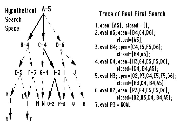
Search Methods • Best-first search • Greedy best-first search • A* search • Hill-climbing search • Genetic algorithms

Best-First Search • Evaluation function f gives cost for each state – Choose state with smallest f(state) (‘the best’) – Agenda: f decides where new states are put – Graph: f decides which node to expand next • Many different strategies depending on f – For uniform-cost search f = path cost – greedy best-first search – A* search

Greedy best-first search • Evaluation function f(n) = h(n) (heuristic) = estimate of cost from n to goal • Ignores the path cost • Greedy best-first search expands the node that appears to be closest to goal

Greedy search • Use as an evaluation function f(n) = h(n) • Selects node to expand believed to be closest (hence “greedy”) to a goal node (i. e. , select node with smallest f value) • as in the example. – Assuming all arc costs are 1, then greedy search will find goal g, which has a solution cost of 5. – However, the optimal solution is the path to goal I with cost 3. a h=2 b g h=4 h=1 c h h=1 d i h=0 h=1 e h=0 g

Romania with step costs in km

Greedy best-first search example

Optimal Path

Greedy Best-First Search Algorithm Input: State Space Ouput: failure or path from a start state to a goal state. Assumptions: L is a list of nodes that have not yet been examined ordered by their h value. The state space is a tree where each node has a single parent. 1. 2. Set L to be a list of the initial nodes in the problem. While L is not empty 1. 2. Pick a node n from the front of L. If n is a goal node 1. stop and return it and the path from the initial node to n. Else 1. remove n from L. 2. For each child c of n 1. insert c into L while preserving the ordering of nodes in L and labelling c with its path from the initial node as well as its h value. End for End if End while Return failure

Properties of greedy best-first search • Complete? – Not unless it keeps track of all states visited • Otherwise can get stuck in loops (just like DFS) • Optimal? – No – we just saw a counter-example • Time? – O(bm), can generate all nodes at depth m before finding solution – m = maximum depth of search space

Uniform Cost Search • Let g(n) be the sum of the edges costs from root to node n. If g(n) is our overall cost function, then the best first search becomes Uniform Cost Search, also known as Dijkstra’s single-source-shortest-path algorithm. • Initially the root node is placed in Open with a cost of zero. At each step, the next node n to be expanded is an Open node whose cost g(n) is lowest among all Open nodes.

Example of Uniform Cost Search • Assume an example tree with different edge costs, represented by numbers next to the edges. a 2 1 c b 1 f Notations for this example: generated node expanded node 2 gc 1 dc 2 ce

Uniform-cost search Sample 0

Uniform-cost search Sample 75 X 140 118

Uniform-cost search Sample 146 X X 140 118

Uniform-cost search Sample 146 X X 140 X 229

Uniform-cost search • Complete? Yes • Time? # of nodes with g ≤ cost of optimal solution, O(bceiling(C*/ ε)) where C* is the cost of the optimal solution • Space? # of nodes with g ≤ cost of optimal solution, O(bceiling(C*/ ε)) • Optimal? Yes

Hill Climbing & Gradient Descent • For artefact-only problems (don’t care about the path) • Depends on some e(state) – Hill climbing tries to maximise score e – Gradient descent tries to minimise cost e (the same strategy!) • Randomly choose a state – Only choose actions which improve e – If cannot improve e, then perform a random restart • Choose another random state to restart the search from • Only ever have to store one state (the present one) – Can’t have cycles as e always improves

Hill-climbing search • Problem: depending on initial state, can get stuck in local maxima

Hill Climbing - Algorithm 1. Pick a random point in the search space 2. Consider all the neighbors of the current state 3. Choose the neighbor with the best quality and move to that state 4. Repeat 2 thru 4 until all the neighboring states are of lower quality 5. Return the current state as the solution state

Example: 8 Queens • Place 8 queens on board – So no one can “take” another • Gradient descent search – Throw queens on randomly – e = number of pairs which can attack each other – Move a queen out of other’s way • Decrease the evaluation function – If this can’t be done • Throw queens on randomly again

Hill-climbing search • Looks one step ahead to determine if any successor is better than the current state; if there is, move to the best successor. • Rule: If Rule: there exists a successor s for the current state n such that • h(s) < h(n) and • h(s) ≤ h(t) for all the successors t of n, then move from n to s. Otherwise, halt at n.

Hill-climbing search • Similar to Greedy search in that it uses h(), but does not allow backtracking or jumping to an alternative path since it doesn’t “remember” where it has been.

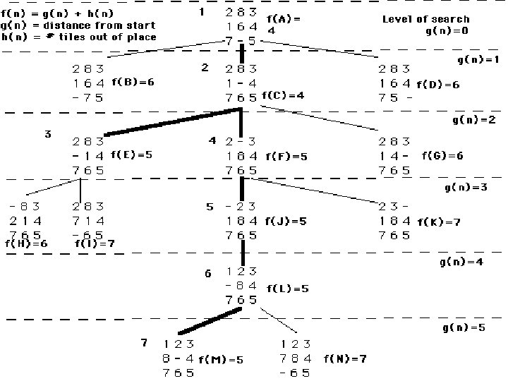
A* Search Algorithm Evaluation function f(n) = h(n) + g(n) h(n) estimated cost to goal from n g(n) cost so far to reach n A* uses admissible heuristics, i. e. , h(n) ≤ h*(n) where h*(n) is the true cost from n. A* Search finds the optimal path 9/24/2021

A* search • Best-known form of best-first search. • Idea: avoid expanding paths that are already expensive. • Combines uniform-cost and greedy search • Evaluation function f(n)=g(n) + h(n) – g(n) the cost (so far) to reach the node – h(n) estimated cost to get from the node to the goal – f(n) estimated total cost of path through n to goal • Implementation: Expand the node n with minimum f(n) 50

A* search example

3 S 2 1 A 6 D 1 B 4 E C try yourself F 8 20 straight-line distances 1 h(S-G)=10 h(A-G)=7 G h(D-G)=1 h(F-G)=1 h(B-G)=10 h(E-G)=8 h(C-G)=20 The graph above shows the step-costs for different paths going from the start (S) to the goal (G). On the right you find the straight-line distances. Draw the search tree for this problem. Avoid repeated states. . 1 Give the order in which the tree is searched (e. g. S-C-B. . . -G) for A* search. . 2 Use the straight-line dist. as a heuristic function, i. e. h=SLD, and indicate for each node visited what the value for the evaluation function, f, is.

$*^$Properties of A • Complete? Yes (unless there are infinitely many nodes with f ≤ f(G) ) • Time? Exponential • Space? Keeps all nodes in memory • Optimal? Yes

start B 2714 200 300 50 630 570 1350 I 1190 700 340 600 P 1841 Q 2848 A 1318 City Map 685 120 890 1220 740 J 1666 780 N 2427 950 1430 W 1974 C 1170 1080 1025 M 725 730 870 775 O 0 K 480 600 goal

B 2714 + 0 2714 Open B Close

Open P N Q Close B B 2714 + 0 200 Q 2848 + 200 3048 630 P 1841 + 630 2471 50 N 2427 + 50 2477

Open I N C Q A W Close B P B 2714 + 0 200 Q 2848 + 200 3048 1350 A 1318 + 1980 3298 50 630 P 1841 + 630 570 685 I 1190 + 1180 2390 C 1170 + 1315 2485 N 2427 + 50 2477 780 W 1974 + 1410 3384

Open N C M Q A W Close B P I B 2714 + 0 200 50 630 P 1841 + 630 Q 2848 + 200 3048 570 685 I 1190 + 1180 700 A 1318 + 1900 3218 C 1170 + 1315 2485 890 M 725 + 2090 2815 N 2427 + 50 2477 780 W 1974 + 1410 3384

Open C M W Q A Close B P I N B 2714 + 0 200 50 630 P 1841 + 630 Q 2848 + 200 3048 570 685 I 1190 + 1200 700 A 1318 + 1900 3218 C 1170 + 1315 2485 890 M 725 + 2090 2815 N 2427 + 50 950 W 1974 + 1000 2974

Open M K W Q A Close B P I N B 2714 + 0 200 50 630 P 1841 + 630 Q 2848 + 200 3048 570 685 I 1190 + 1180 700 A 1318 + 1900 3218 C 1170 + 1315 890 M 725 + 2090 2815 N 2427 + 50 950 W 1974 + 1000 2974 1025 K 480 + 2340 2820

Open K O W Q A J Close B P I N M B 2714 + 0 200 50 630 N 2427 + 50 P 1841 + 630 Q 2848 + 200 3048 570 685 I 1190 + 1180 700 A 1318 + 1900 3218 950 C 1170 + 1315 890 740 J 1666 + 2830 4496 M 725 + 2090 870 W 1974 + 1000 2974 1025 K 480 + 2340 2820 O 0 + 2960

Open O W Q A J Close B P I N M K B 2714 + 0 200 50 630 N 2427 + 50 P 1841 + 630 Q 2848 + 200 3048 570 685 I 1190 + 1180 700 A 1318 + 1900 3218 J 1666 + 2830 4496 W 1974 + 1000 2974 1025 K 600 480 + 2340 C 1170 + 1315 890 740 950 M 725 + 2090 O 0 + 2940

Open O W Q A J Close B P I N M K B 2714 + 0 630 P 1841 + 630 685 C 1170 + 1315 1025 K 600 480 + 2340 O 0 + 2940

IDA* Search • Problem with A* search – You have to record all the nodes – In case you have to back up from a dead-end • A* searches often run out of memory, not time • Use the same iterative deepening trick as IDS – But iterate over f(state) rather than depth – Define contours: f < 100, f < 200, f < 300 etc. • Complete & optimal as A*, but less memory

IDA* Search: Contours • Find all nodes – Where f(n) < 100 – Ignore f(n) >= 100 • Find all nodes – Where f(n) < 200 – Ignore f(n) >= 200 • And so on…

Genetic algorithms • A successor state is generated by combining two parent states • Start with k randomly generated states (population) • A state is represented as a string over a finite alphabet (often a string of 0 s and 1 s) • Evaluation function (fitness function). Higher values for better states. • Produce the next generation of states by selection, crossover, and mutation

Genetic algorithms • Fitness function: number of non-attacking pairs of queens (min = 0, max = 8 × 7/2 = 28) • 24/(24+23+20+11) = 31% • 23/(24+23+20+11) = 29% etc

Mutation • Mutation randomly changes genes in the new offspring. • For binary encoding we can switch a few randomly chosen bits from 1 to 0 or from 0 to 1. Original offspring Mutated offspring 1101111000011110 1100111000001110

Class Exercise: Local Search for Map/Graph Coloring

G(n) = The cost of each move as the distance between each town (shown on map). H(n) = The Distance between any town and town M. (START) A 36 B 61 31 L C 80 32 D 52 E 31 43 F 112 G 20 102 K 122 H 32 36 40 I 45 M (END) J

Search Strategies Uninformed • Breadth-first search • Depth-first search • Iterative deepening • Bidirectional search • Uniform-cost search Informed • Greedy search • A* search • IDA* search • Hill climbing

G(n) = The cost of each move as the distance between each town H(n) = The Straight Line Distance between any town and town M. A 40 12 20 C D 10 23 5 I 10 15 20 10 G 10 K 10 5 F E B L 10 20 H J 5 M A 45 E 32 I 12 B 20 F 23 J 5 C 34 G 15 K 40 D 25 H 10 L 20 M 0

• Consider the following search problem. Assume a state is represented as an integer, that the initial state is the number 1, and that the two successors of a state n are the states 2 n and 2 n+1. For example, the successors of 1 are 2 and 3, the successors of 2 are 4 and 5, the successors of 3 are 6 and 7, etc. Assumes the goal state is the number 12. Consider the following heuristics for evaluating the state n where the goal state is g • h 1(n) = |n-g| & h 2(n) = (g – n) if (n g) and h 2 (n) = if (n >g) • Show the search trees generated for each of the following strategies for the initial state 1 and the goal state 12, numbering the nodes in the order expanded. • Depth-first search b) Breadth-first search • c) beast-first with heuristic h 1 d) A* with heuristic (h 1+h 2) • If any of these strategies get lost and never find the goal, then show the few steps and say "FAILS"

The end!