approximating graph spanners Guy Kortsarz Rutgers Camden Unweighted

approximating graph spanners Guy Kortsarz, Rutgers Camden

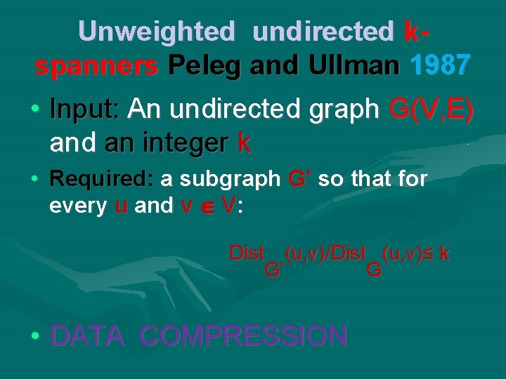
Unweighted undirected kspanners Peleg and Ullman 1987 • Input: An undirected graph G(V, E) and an integer k • Required: a subgraph G’ so that for every u and v V: Dist (u, v)/Dist (u, v)≤ k G’ G • DATA COMPRESSION

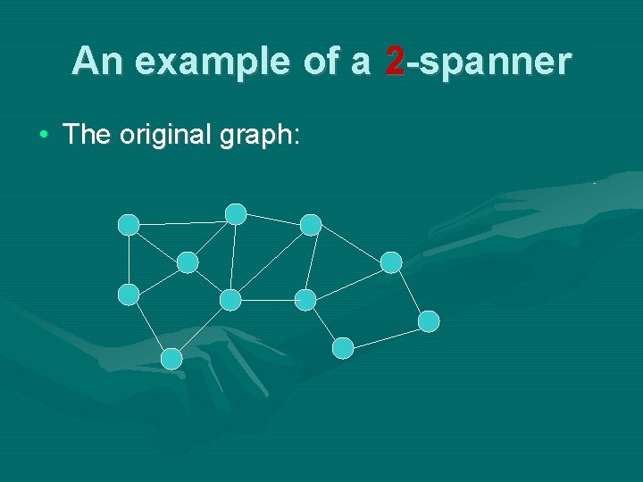
An example of a 2 -spanner • The original graph:

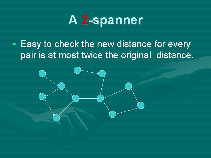
A 2 -spanner • Easy to check the new distance for every pair is at most twice the original distance.

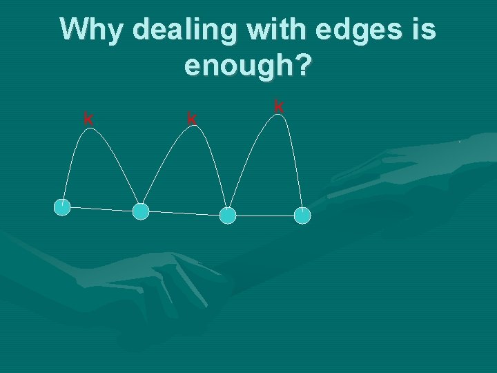
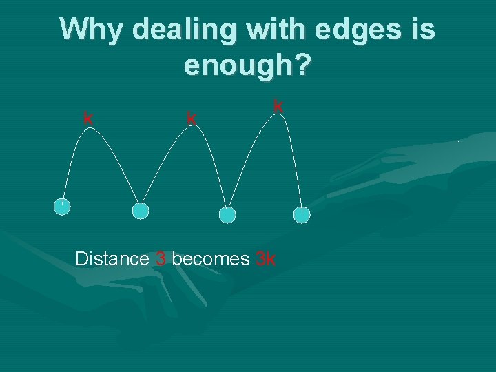
Why dealing with edges is enough? k k k

Why dealing with edges is enough? k k k Distance 3 becomes 3 k

An alternative definition • Find a subgraph G’(V, E’) so that for every edge e in E-E’, adding e must close a cycle of size at most k+1. • More general variants in which the above is not true. • The case of general lengths over the edges. • Then a k-spanner must be a k-spanner with respect to weighted distance.

Applications • In geometry. • Small routing tables: spanners have less edges. Thus smaller tables. But not much larger distance • Synchronizers: make non synchronized distributed computation, synchronized. • Parallel distributed and streaming algorithms. • Distance oracles. Handle queries about distance between two vertices quick by preprocessing. • Property testing • Minimum time broadcast.

2 -spanners • There is a difficulty. Unlike k≥ 3 there are not necessarily 2 spanners with few edges. • The only 2 -spanners of a complete bipartite graph is the graph itself. • Like in 2 -SAT and 2 -Coloring and other problems, 2 -spanners is different than the rest.

For k at least 3 there are spanners with few edges • As we shall see: 3 -spanners with O(n*sqrt{n}) edges always exist, and the same goes for 4 -spanners. And this is tight. • The larger k is, the smaller is the upper bound on the number of edges in the best spanner. • Remarkable fact: maximum number of edges in a graph with girth g not known.

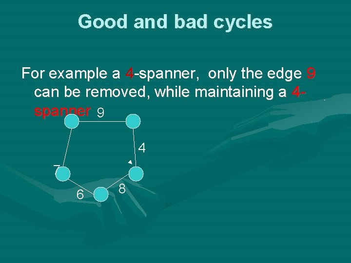
Good and bad cycles For example a 4 -spanner, only the edge 9 can be removed, while maintaining a 4 spanner 9 4 7 6 8

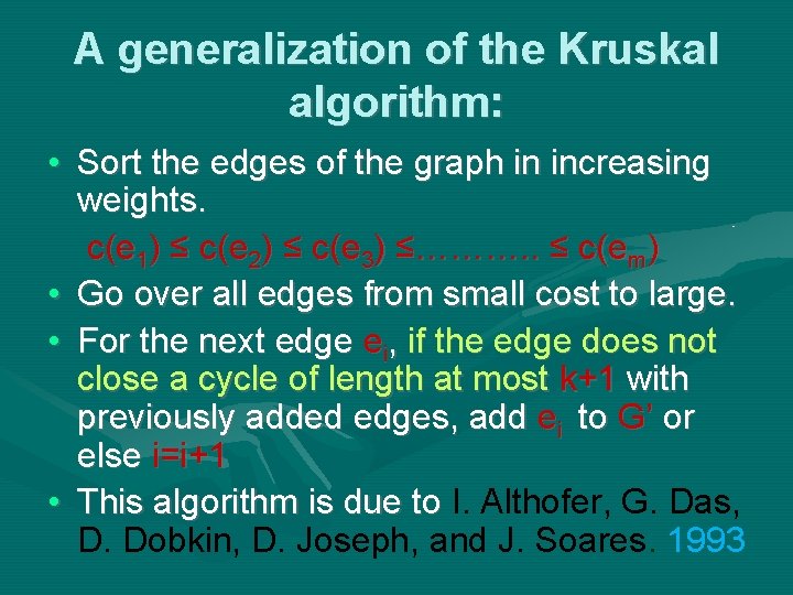
A generalization of the Kruskal algorithm: • Sort the edges of the graph in increasing weights. c(e 1) ≤ c(e 2) ≤ c(e 3) ≤………. . ≤ c(em) • Go over all edges from small cost to large. • For the next edge ei, if the edge does not close a cycle of length at most k+1 with previously added edges, add ei to G’ or else i=i+1 • This algorithm is due to I. Althofer, G. Das, D. Dobkin, D. Joseph, and J. Soares. 1993

The resulting graph is a kspanner • If an edge e is missing, then by construction, this edge is the most heavy edge in a cycle of length at most k+1. • This is because we go over edges in non decreasing costs. • If we reach a cycle of size k+1, then it means that previous edges were not removed. • This implies that e is the largest edge in a cycle of length at most k+1 and it is safe to remove it.

Girth k+2 • We observe that the resulting graph has girth at least k+2 • The girth is the size of the minimum simple cycle. • Observe that when we reach the largest edge e of a cycle with at most k+1 edges it will be removed. • Therefore, there are no k+1 size or smaller cycles. • Graphs with large girth have “few’’ edges.

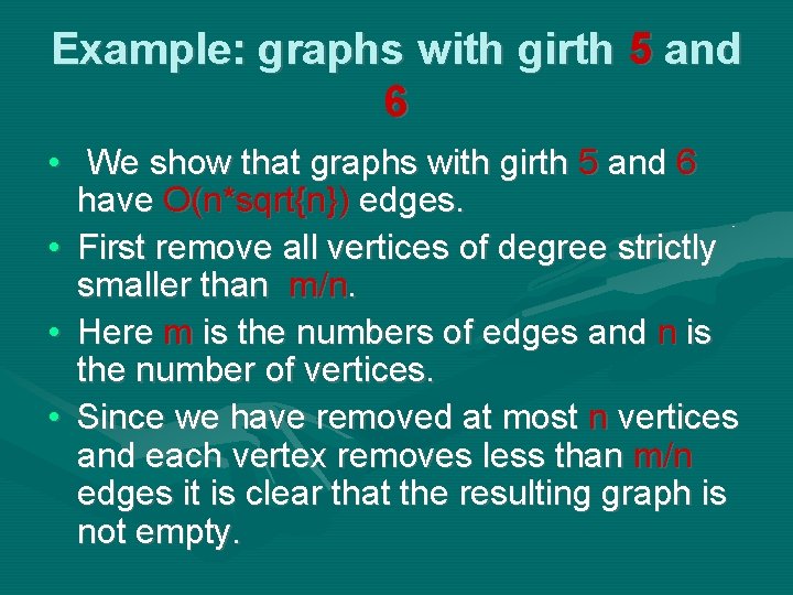
Example: graphs with girth 5 and 6 • We show that graphs with girth 5 and 6 have O(n*sqrt{n}) edges. • First remove all vertices of degree strictly smaller than m/n. • Here m is the numbers of edges and n is the number of vertices. • Since we have removed at most n vertices and each vertex removes less than m/n edges it is clear that the resulting graph is not empty.

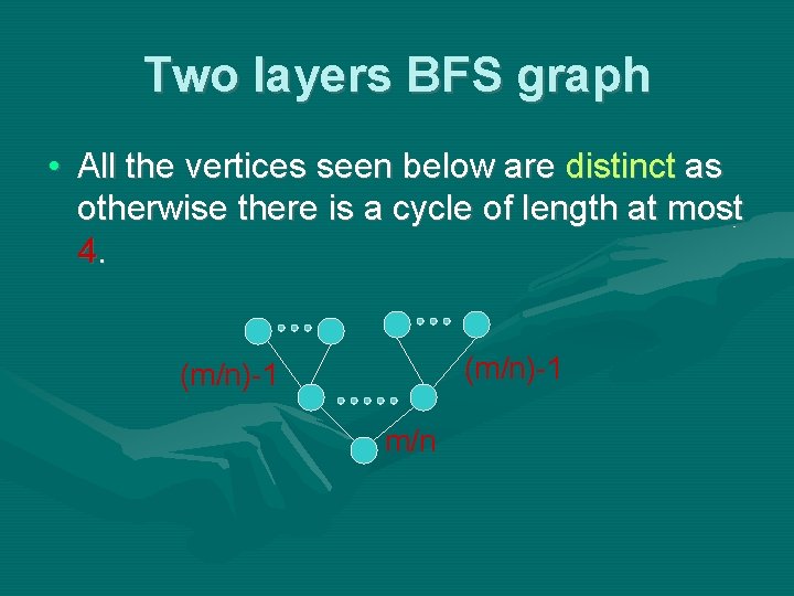
Two layers BFS graph • All the vertices seen below are distinct as otherwise there is a cycle of length at most 4. (m/n)-1 m/n

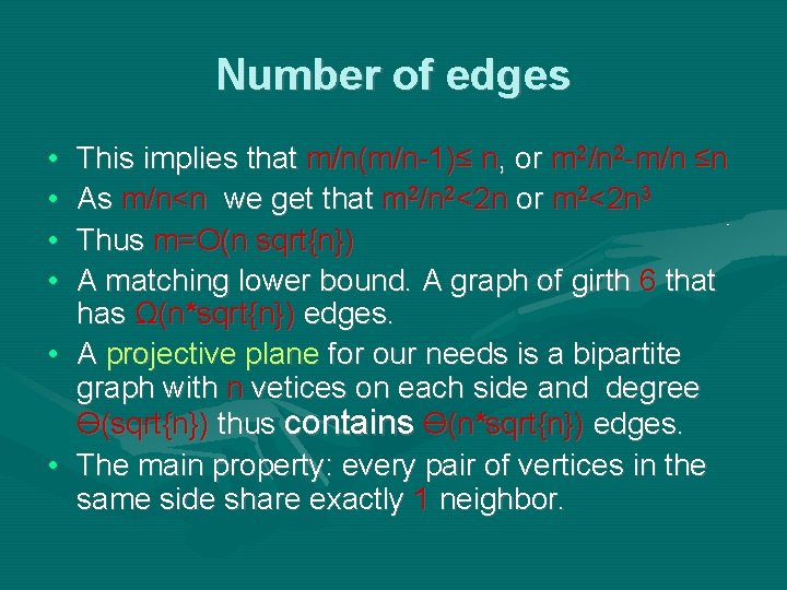
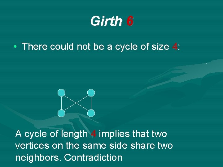
Number of edges • • This implies that m/n(m/n-1)≤ n, or m 2/n 2 -m/n ≤n As m/n<n we get that m 2/n 2<2 n or m 2<2 n 3 Thus m=O(n sqrt{n}) A matching lower bound. A graph of girth 6 that has Ω(n*sqrt{n}) edges. • A projective plane for our needs is a bipartite graph with n vetices on each side and degree Ө(sqrt{n}) thus contains Ө(n*sqrt{n}) edges. • The main property: every pair of vertices in the same side share exactly 1 neighbor.

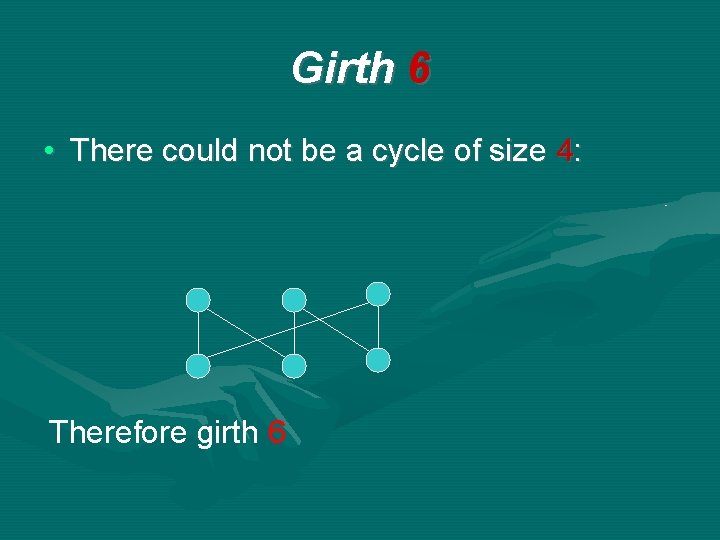
Girth 6 • There could not be a cycle of size 4: A cycle of length 4 implies that two vertices on the same side share two neighbors. Contradiction

Girth 6 • There could not be a cycle of size 4: Therefore girth 6

General bounds on the minimum number of edges for a given girth • It is known that there is always a 2 k-1 spanner with O(n 1+1/k) edges. • Using this formula: 3 -spanners needs k=2. This gives the correct and tight O(n* sqrt{n}) upper bound on the number of edges in a 3 -spanner. • Approximation? O(log d) approximation with d the average degree for minimum cost 2 -spanners (but lengths 1). • As we shall see such an approximation does not exist for k≥ 3.

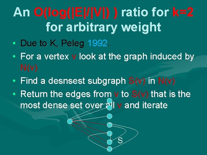
An O(log(|E|/|V|) ) ratio for k=2 for arbitrary weight • Due to K, Peleg 1992. • For a vertex v look at the graph induced by N(v) • Find a desnsest subgraph S(v) in N(v) • Return the edges from v to S(v) that is the most dense set over all v and iterate S

The problem we need to solve is the densest subgraph • Let e(S), S N(v) be the number of edges in the graph induced by S. • This problem requires finding a subset of the vertices with maximum density e(S)/|S| and can be solved exactly via flow. This implies an O(log d) ratio for d the average degree. • A faster algorithm, approximates the best density by 2 but get O(n) time and not flow time. Adds 2 to the ratio (so negligible). • Was done by K, Peleg in 1992. Also Charikar 1998. • Very extensively cited in social networks. Almost always attribute the result to Charikar.

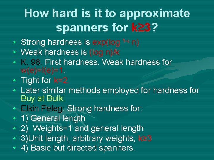
How hard is it to approximate spanners for k≥ 3? • • • Strong hardness is exp(log 1 - n) Weak hardness is (log n)/k K. 98. First hardness. Weak hardness for w(e)=l(e)=1. Tight for k=2. Later similar methods employed for hardness for Buy at Bulk. Elkin Peleg: Strong hardness for: 1) General length 2) Weights=1 and general length 3)Unit length, arbitrary weights, k≥ 3 4) Basic but directed spanners.

Only basic spanners from now on • From now on, edges have weights and lengths 1. • Thus the results presented from now on are only for basic spanners. • In fact giving a similar result for arbitrary weights already unknown for some of the problems in later slides. • And none of the algorithms to follow work on general lengths.

A question posed in 1992 • Is undirected the basic spanner problem strongly hard? • In ICALP 2012 Dinitz, K, Raz : k≥ 3 is Labelcover-Hard (means only polynomial ratio is possible). • Second important result: Labelcover with large girth is as hard as Labelcover • Its rare (for me) to solve a 20 years old problem.

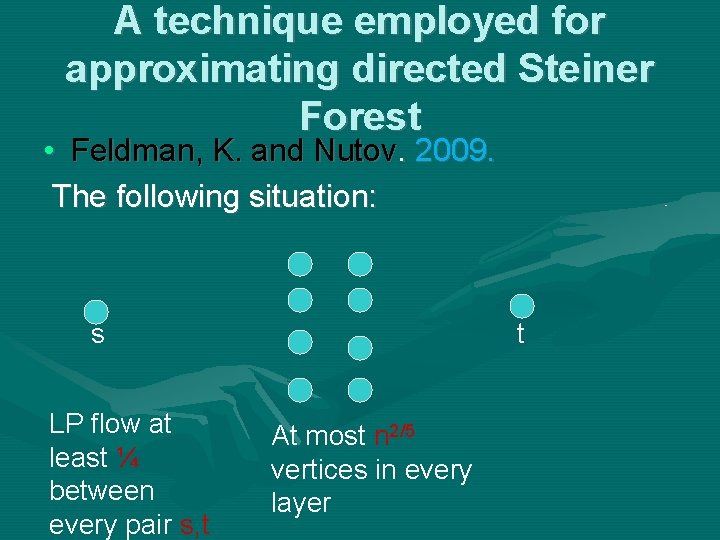
A technique employed for approximating directed Steiner Forest • Feldman, K. and Nutov. 2009. The following situation: s LP flow at least ¼ between every pair s, t t At most n 2/5 vertices in every layer

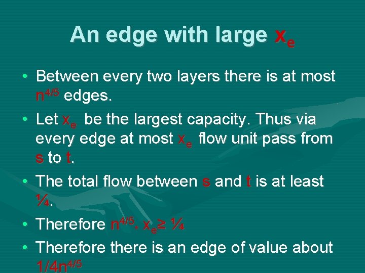
An edge with large xe • Between every two layers there is at most n 4/5 edges. • Let xe be the largest capacity. Thus via every edge at most xe flow unit pass from s to t. • The total flow between s and t is at least ¼. • Therefore n 4/5* xe≥ ¼ • Therefore there is an edge of value about 1/4 n 4/5

Approximating directed spanners • Krauthgamer and Dinitz 2012, employed (part of) our techniques to get an n 2/3 approximation for directed k-spanners. The techniques was (re)invented independently. • Improvement: non iterative but randomized rounding gets about n 1/2 ratio. Very clever trick! • Due to Berman, Bhattacharyya, Makarychev, Raskhodnikova, Yaroslavtsev. 2013.

Other results • For k=3 they get ratio n 1/3 ratio for the directed case. Note that even for undirected graphs n 1/2 is trivial but n 1/3 not. • They also improve the result for Directed Steiner forest. The new best ratio is n 2/3. • Can we show a better integrality gap for the natural LP? • The answer is no.

Dinitz and Zhang 2016 • Ratio n 1/3 for k=4 • The ADDJ upper bound and the integrality gaps of the natural LP are not that far. • Interesting proof: builds its own type of Min -Rep and uses the fact that Min-Rep is hard for large super girth several times. • I would guess that the ratio of ADDJ will not be easily improved if at all.

Preservers • The input contains a collection of pairs {x, y} and you want minimum edges G’ so that the distance between every x, y is the same as in G. • A paper by Chlamtac, Dinitz, K, and Laekhanukit, SODA 2017. • Ratio O(n 3/5 ) approximation for preservers. • There is a big problem. The inequality opt≥n-1 does not hold.

How to overcome this • The SODA 2017 paper introduced junction trees at the last stage. • Junction trees are trees that connect many s, t pairs so that all paths from s, t for every pair goes via the same vertex r. • Invented in relation to Buy at Bulk. • Namely when the relative cost of items goes down if you buy many.

Why do the junction trees help • Instead of bounding the cost by n-1 you bound the cost by the number of terminal pairs connected, times the maximum length. • It has some small tricks like applying a different algorithm if the number of pairs is Ω(n 4/5 ).

Approximation Steiner Forest with distance bounds • Input: Given the pairs{s, t} each pair has a distance bound D(s, t) • Objective: find a minimum cost solution so that the distance between every pair of vertices s, t is at most D(s, t). • The same approximation ratio: O(n 3/5 )

Getting back to Directed Steiner Forest • First sub-linear ratio by Feldman, Kortsarz, Nutov , 2009, O(n 4/5 ). • Berman et al, 2013, improved the ratio to O(n 2/3 ) using their clever randomized rounding method. • Using our additional junction tree and threshold trick we improve Berman et al to O(n 3/5 ) (however recall that our result is for the unweighted case). SODA 2017.

The message of this last paper • Introducing junction tress can help approximating spanner problems. The first time junction trees ever used in spanners. • A second message is that it seems that additive spanners are harder to approximate than usual spanners.

Additive spanners • Aingworth, Chekuri, Indyk, Motwani 1996. For any graph, n∙ sqt{n} edges +2 spanners. • Chechik. +4 spanners always exists with O(n 7/5 ) 2013. • Baswana, Kavitha, Mehlhorn, Pettie show: Always exists +6, O(n 4/3) 2010 (before +4). • Can we continue with this hobby for k=8, k=10 and so on?

Surprise (at least for me) • • • Amir Abboud and Greg Bodwin. 2016 The O(n 4/3) can not be improved. There are large µ, so that µ, additive spanners requires Ω(n 4/3) edges. • The last result for k=6 is best possible for much higher k. • How do additive spanners compare to spanners for approximation? Turns out: Also harder.

The case of k=1 • We gave the first lower bound. SODA 2017. • If we have edges of cost 0 this is easy. • We can not show that its hard to spann edges because of the O(log n) for k=2. • Dividing edges brings new edges that need to be spanned. Feels like catch 22. • Overcoming that by making the new paths added the same Labelcover hard. CDLK, SODA 2017.

For k=O(polylog(n)) • Again Labercover hard. Harder proof. • Additive spanners are harder to aproximate that spanners. • Any +1 spanner is a 2 -spanner but +1 spanner much harder • Also O(log n) spanner has constant ratio but additive polylog(n) spanner is Labelcover hard. • The +1 spanners result surprised me.

Open problems • Transitive closure spanners. Tree spanners • Fault tolerant spanners. Simple and nice Algorithm by Dinitz and Krauthgamer. • Fault tolerant spanners: new version • Preserve the distance from s to G-s under at most f edges that can fall. Peleg Parver. • Find a minimum H so that for any |F|≤f, dist(s, u, G-F)=dist(s, u, H-F). Turned to be equivalent to Set Cover. Peleg Parver. • Many open questions remain here.

It is not possible to predict the future. Did you know that? • Peleg and Ulman invented spanners in 1987. • There was nothing. Only some results from geometry. • I would imagine Peleg and Ulman did not expect the extent of which this subject will develop back then.