Antenna Theory and Design Associate Professor WANG Junjun

Antenna Theory and Design Associate Professor WANG Junjun 王珺珺 School of Electronic and Information Engineering Beihang University wangjunjun@buaa. edu. cn 13426405497 New Main Building F 1025 1

Chapter 4 Wire Antennas

Chapter 4 Wire Antennas ▫ ▫ ▫ ▫ Infinitesimal Dipole Small Dipole Finite length Dipole Half-wavelength Dipole Antenna above a perfect ground plane Folded Dipole Yagi Uda Antenna Travelling-Wave Antenna

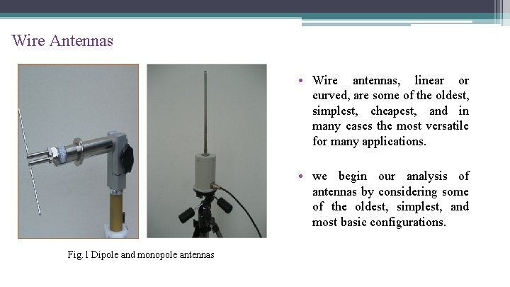
Wire Antennas • Wire antennas, linear or curved, are some of the oldest, simplest, cheapest, and in many cases the most versatile for many applications. • we begin our analysis of antennas by considering some of the oldest, simplest, and most basic configurations. Fig. 1 Dipole and monopole antennas

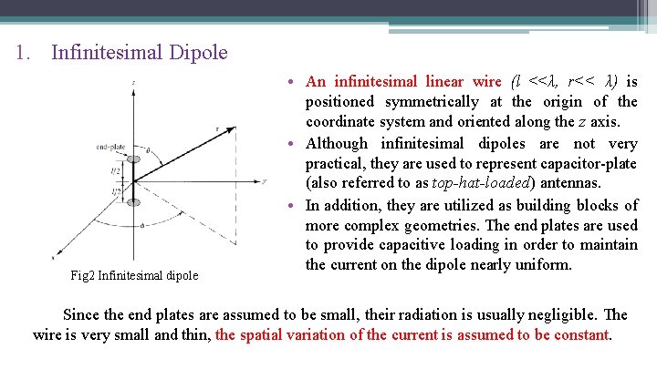
1. Infinitesimal Dipole Fig 2 Infinitesimal dipole • An infinitesimal linear wire (l <<λ, r<< λ) is positioned symmetrically at the origin of the coordinate system and oriented along the z axis. • Although infinitesimal dipoles are not very practical, they are used to represent capacitor-plate (also referred to as top-hat-loaded) antennas. • In addition, they are utilized as building blocks of more complex geometries. The end plates are used to provide capacitive loading in order to maintain the current on the dipole nearly uniform. Since the end plates are assumed to be small, their radiation is usually negligible. The wire is very small and thin, the spatial variation of the current is assumed to be constant.

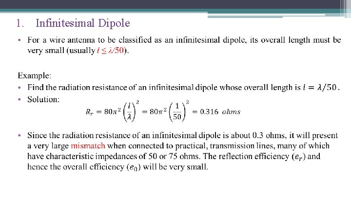
1. Infinitesimal Dipole • The radiation resistance is: • The input reactance is capacitive. • This can be seen by visualizing the antenna as an open circuited transmission line. The distance from the end of the antenna to the feed point is much less than a quarter Fig 3 Three-dimensional radiation pattern wavelength and thus the input impedance is of infinitesimal dipole capacitive. • The maximum effective aperture: • The directivity of this antenna:

1. Infinitesimal Dipole

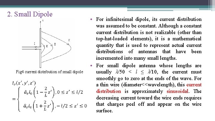
2. Small Dipole Fig 4 current distribution of small dipole • For infinitesimal dipole, its current distribution was assumed to be constant. Although a constant current distribution is not realizable (other than top-hat-loaded elements), it is a mathematical quantity that is used to represent actual current distributions of antennas that have been incremented into many small lengths. • For small dipole antenna whose lengths are usually λ/50 < l ≤ λ/10, the current must smoothly go to zero at the ends of the wave. For a thin wire (diameter<<wavelength), this current distribution is approximately sinusoidal. The decreasing current toward the wire ends requires that charges peel off and appear on the wire surface.

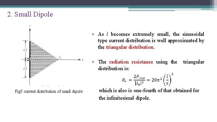
2. Small Dipole • As l becomes extremely small, the sinusoidal type current distribution is well approximated by the triangular distribution. • The radiation resistance using the triangular distribution is: Fig 5 current distribution of small dipole which is also is one-fourth of that obtained for the infinitesimal dipole.

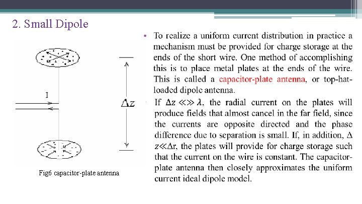
2. Small Dipole Fig 6 capacitor-plate antenna

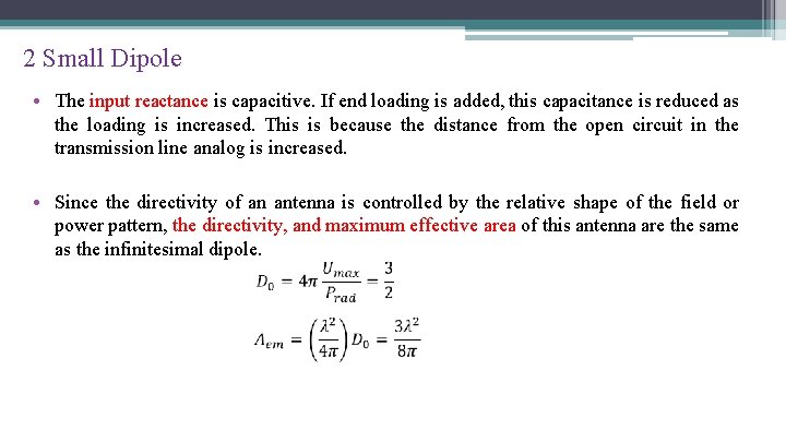
2 Small Dipole • The input reactance is capacitive. If end loading is added, this capacitance is reduced as the loading is increased. This is because the distance from the open circuit in the transmission line analog is increased. • Since the directivity of an antenna is controlled by the relative shape of the field or power pattern, the directivity, and maximum effective area of this antenna are the same as the infinitesimal dipole.

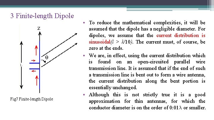
3 Finite-length Dipole Fig 7 Finite-length Dipole • To reduce the mathematical complexities, it will be assumed that the dipole has a negligible diameter. For dipoles, we assume that the current distribution is sinusoidal(l > λ/10). The current must, of course, be zero at the ends. • We are, in effect, using the current distribution which is found on an open-circuited parallel wire transmission line. It is assumed that if the end of such a transmission line is bent out to form a wire antenna, the current distribution along the bent portion is essentially unchanged. • Although this is not strictly true it is a good approximation for thin antennas, for which the conductor diameter is on the order of 0: 01 or smaller.

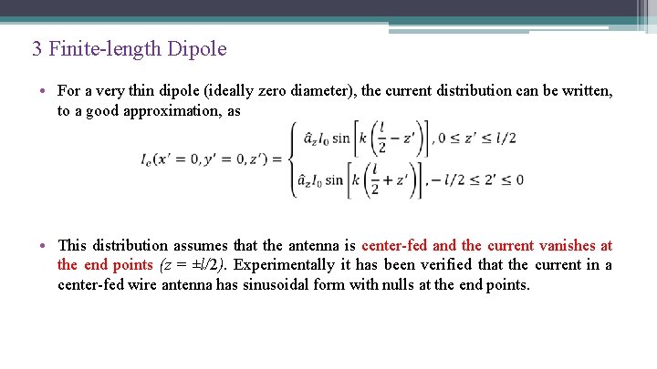
3 Finite-length Dipole • For a very thin dipole (ideally zero diameter), the current distribution can be written, to a good approximation, as • This distribution assumes that the antenna is center-fed and the current vanishes at the end points (z = ±l/2). Experimentally it has been verified that the current in a center-fed wire antenna has sinusoidal form with nulls at the end points.

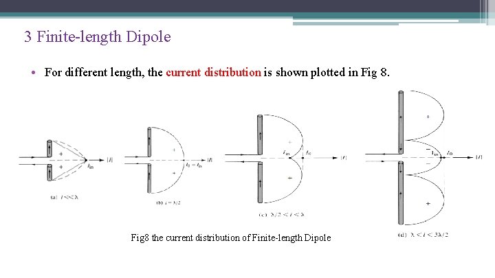
3 Finite-length Dipole • For different length, the current distribution is shown plotted in Fig 8 the current distribution of Finite-length Dipole

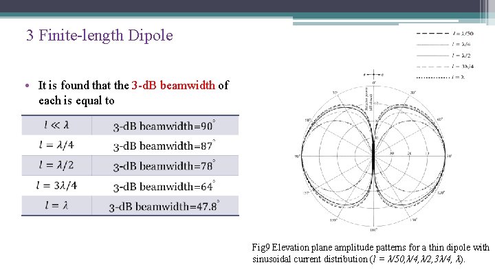
3 Finite-length Dipole • It is found that the 3 -d. B beamwidth of each is equal to Fig 9 Elevation plane amplitude patterns for a thin dipole with sinusoidal current distribution (l = λ/50, λ/4, λ/2, 3λ/4, λ).

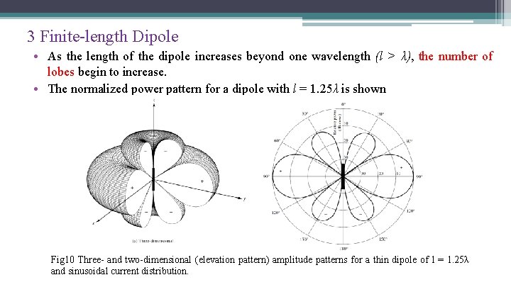
3 Finite-length Dipole • As the length of the dipole increases beyond one wavelength (l > λ), the number of lobes begin to increase. • The normalized power pattern for a dipole with l = 1. 25λ is shown Fig 10 Three- and two-dimensional (elevation pattern) amplitude patterns for a thin dipole of l = 1. 25λ and sinusoidal current distribution.

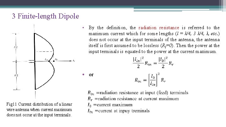
3 Finite-length Dipole • By the definition, the radiation resistance is referred to the maximum current which for some lengths (l = λ/4, 3 λ/4, λ, etc. ) does not occur at the input terminals of the antenna, the antenna itself is first assumed to be lossless (Rl=0). Then the power at the input terminals is equated to the power at the current maximum. • or Fig 11 Current distribution of a linear wire antenna when current maximum does not occur at the input terminals.

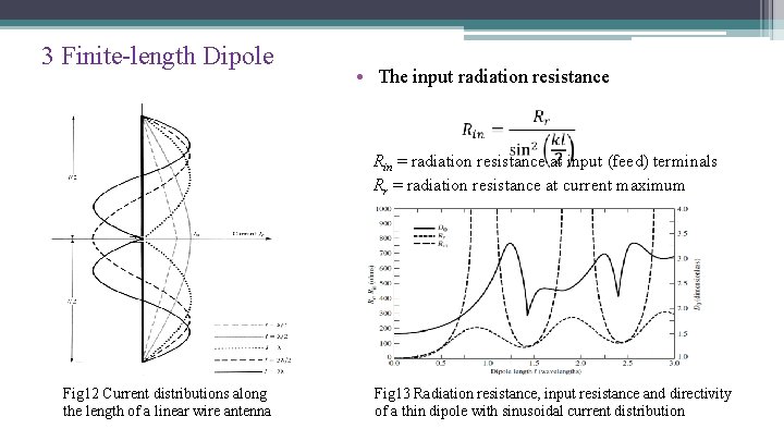
3 Finite-length Dipole • The input radiation resistance Rin = radiation resistance at input (feed) terminals Rr = radiation resistance at current maximum Fig 12 Current distributions along the length of a linear wire antenna Fig 13 Radiation resistance, input resistance and directivity of a thin dipole with sinusoidal current distribution

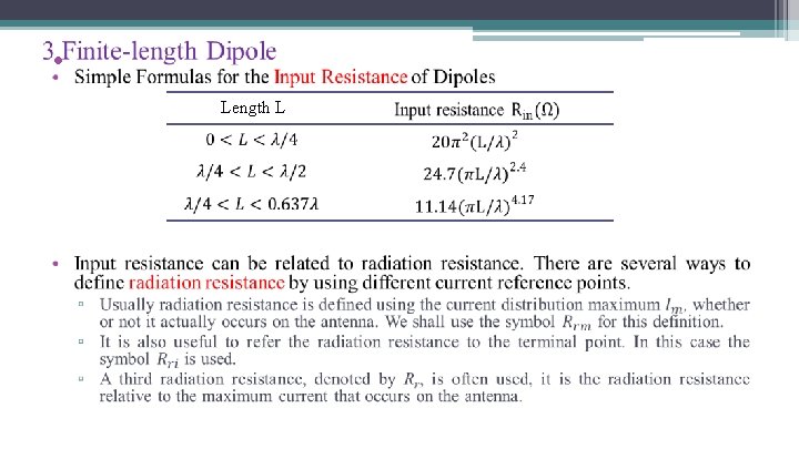
• Length L

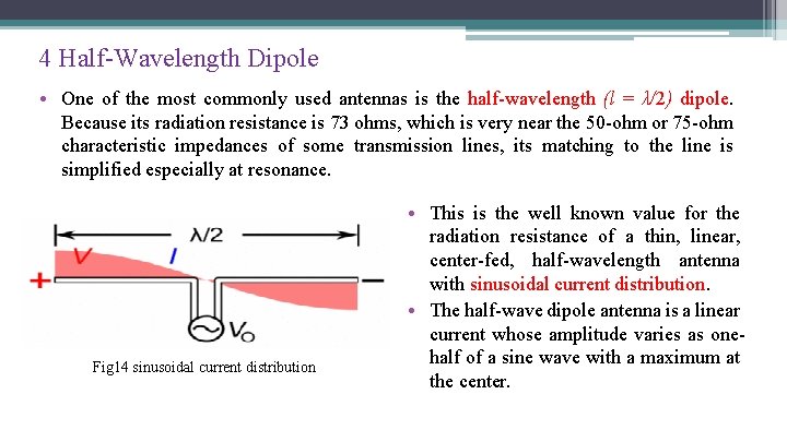
4 Half-Wavelength Dipole • One of the most commonly used antennas is the half-wavelength (l = λ/2) dipole. Because its radiation resistance is 73 ohms, which is very near the 50 -ohm or 75 -ohm characteristic impedances of some transmission lines, its matching to the line is simplified especially at resonance. Fig 14 sinusoidal current distribution • This is the well known value for the radiation resistance of a thin, linear, center-fed, half-wavelength antenna with sinusoidal current distribution. • The half-wave dipole antenna is a linear current whose amplitude varies as onehalf of a sine wave with a maximum at the center.

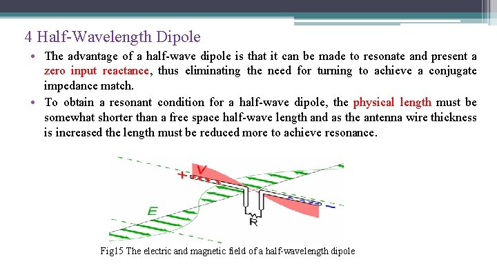
4 Half-Wavelength Dipole • The advantage of a half-wave dipole is that it can be made to resonate and present a zero input reactance, thus eliminating the need for turning to achieve a conjugate impedance match. • To obtain a resonant condition for a half-wave dipole, the physical length must be somewhat shorter than a free space half-wave length and as the antenna wire thickness is increased the length must be reduced more to achieve resonance. Fig 15 The electric and magnetic field of a half-wavelength dipole

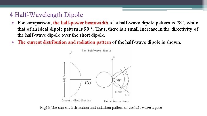
4 Half-Wavelength Dipole • For comparison, the half-power beamwidth of a half-wave dipole pattern is 78 , while that of an ideal dipole pattern is 90 . Thus, there is a small increase in the directivity of the half-wave dipole over the short dipole. • The current distribution and radiation pattern of the half-wave dipole is shown. Fig 16 The current distribution and radiation pattern of the half-wave dipole

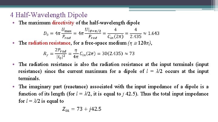
4 Half-Wavelength Dipole • The maximum directivity of the half-wavelength dipole • The radiation resistance, for a free-space medium (η 120π), • The radiation resistance is also the radiation resistance at the input terminals (input resistance) since the current maximum for a dipole of l = λ/2 occurs at the input terminals. • The imaginary part (reactance) associated with the input impedance of a dipole is a function of its length (for l = λ/2, it is equal to j 42. 5). Thus the total input impedance for l = λ/2 is equal to

4 Half-Wavelength Dipole • To reduce the imaginary part of the input impedance to zero, the antenna is matched or reduced in length until the reactance vanishes. The latter is most commonly used in practice for half-wavelength dipoles. To make the reactance zero, requires that the antenna be shorted a few percent less than half-wavelength. This shortening results in a reduction in the value of the radiation resistance to about 65 ohm. • Depending on the radius of the wire, the length of the dipole for first resonance is about l = 0. 47λ to 0. 48λ; the thinner the wire, the closer the length is to 0. 48λ. Thus, for thicker wires, a larger segment of the wire has to be removed from λ/2 to achieve resonance.

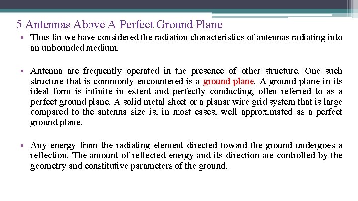
5 Antennas Above A Perfect Ground Plane • Thus far we have considered the radiation characteristics of antennas radiating into an unbounded medium. • Antenna are frequently operated in the presence of other structure. One such structure that is commonly encountered is a ground plane. A ground plane in its ideal form is infinite in extent and perfectly conducting, often referred to as a perfect ground plane. A solid metal sheet or a planar wire grid system that is large compared to the antenna size is, in most cases, well approximated as a perfect ground plane. • Any energy from the radiating element directed toward the ground undergoes a reflection. The amount of reflected energy and its direction are controlled by the geometry and constitutive parameters of the ground.

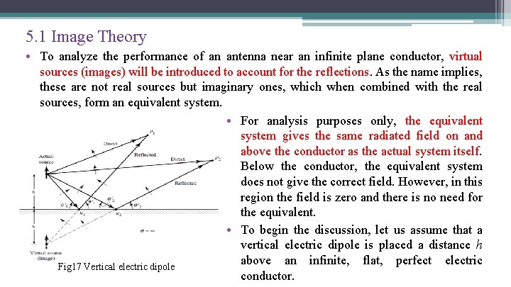
5. 1 Image Theory • To analyze the performance of an antenna near an infinite plane conductor, virtual sources (images) will be introduced to account for the reflections. As the name implies, these are not real sources but imaginary ones, which when combined with the real sources, form an equivalent system. • For analysis purposes only, the equivalent system gives the same radiated field on and above the conductor as the actual system itself. Below the conductor, the equivalent system does not give the correct field. However, in this region the field is zero and there is no need for the equivalent. • To begin the discussion, let us assume that a vertical electric dipole is placed a distance h above an infinite, flat, perfect electric Fig 17 Vertical electric dipole conductor.

5. 1 Image Theory • The amount of reflection is generally determined by the respective constitutive parameters of the media below and above the interface. For a perfect electric conductor below the interface, the incident wave is completely reflected and the field below the boundary is zero. According to the boundary conditions, the tangential components of the electric field must vanish at all points along the interface. • Thus for an incident electric field with vertical polarization shown by the arrows, the polarization of the reflected waves must be as indicated in the figure to satisfy the boundary conditions. To excite the polarization of the reflected waves, the virtual source must also be vertical and with a polarity in the same direction as that of the actual source (thus a reflection coefficient of +1).

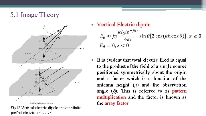
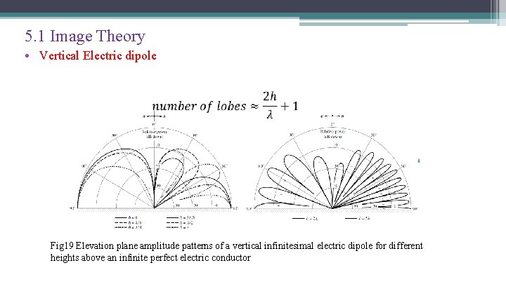
5. 1 Image Theory • Vertical Electric dipole Fig 18 Vertical electric dipole above infinite perfect electric conductor • It is evident that total electric filed is equal to the product of the field of a single source positioned symmetrically about the origin and a factor which is a function of the antenna height (h) and the observation angle ( ). This is referred to as pattern multiplication and the factor is known as the array factor.

5. 1 Image Theory • Vertical Electric dipole Fig 19 Elevation plane amplitude patterns of a vertical infinitesimal electric dipole for different heights above an infinite perfect electric conductor

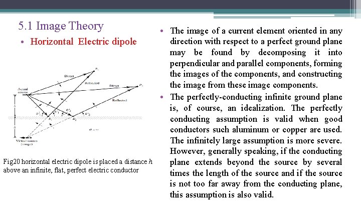
5. 1 Image Theory • Horizontal Electric dipole Fig 20 horizontal electric dipole is placed a distance h above an infinite, flat, perfect electric conductor • The image of a current element oriented in any direction with respect to a perfect ground plane may be found by decomposing it into perpendicular and parallel components, forming the images of the components, and constructing the image from these image components. • The perfectly-conducting infinite ground plane is, of course, an idealization. The perfectly conducting assumption is valid when good conductors such aluminum or copper are used. The infinitely large assumption is more severe. However, generally speaking, if the conducting plane extends beyond the source by several times the length of the source and if the source is not too far away from the conducting plane, this assumption is also valid.

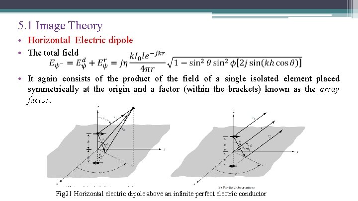
5. 1 Image Theory • Horizontal Electric dipole • The total field • It again consists of the product of the field of a single isolated element placed symmetrically at the origin and a factor (within the brackets) known as the array factor. Fig 21 Horizontal electric dipole above an infinite perfect electric conductor

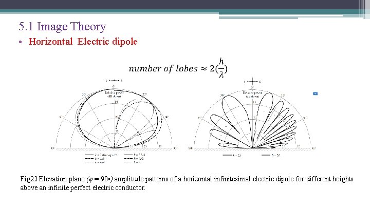
5. 1 Image Theory • Horizontal Electric dipole Fig 22 Elevation plane (φ = 90◦) amplitude patterns of a horizontal infinitesimal electric dipole for different heights above an infinite perfect electric conductor.

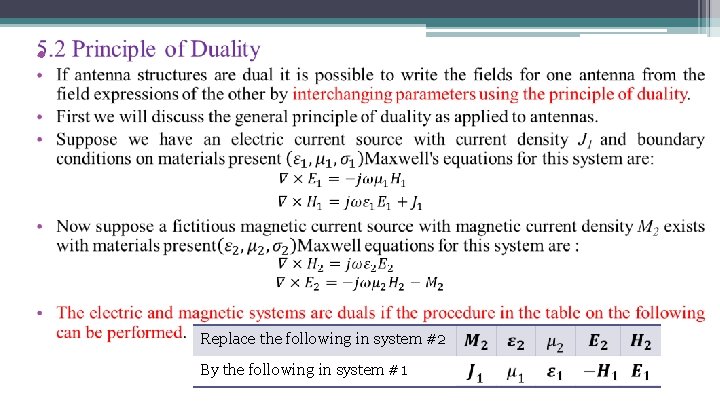
• Replace the following in system #2 By the following in system #1

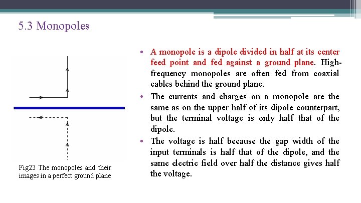
5. 3 Monopoles Fig 23 The monopoles and their images in a perfect ground plane • A monopole is a dipole divided in half at its center feed point and fed against a ground plane. Highfrequency monopoles are often fed from coaxial cables behind the ground plane. • The currents and charges on a monopole are the same as on the upper half of its dipole counterpart, but the terminal voltage is only half that of the dipole. • The voltage is half because the gap width of the input terminals is half that of the dipole, and the same electric field over half the distance gives half the voltage.

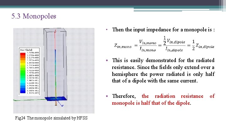
5. 3 Monopoles • Then the input impedance for a monopole is : • This is easily demonstrated for the radiated resistance. Since the fields only extend over a hemisphere the power radiated is only half that of a dipole with the same current. • Therefore, the radiation resistance of monopole is half that of the dipole. Fig 24 The monopole simulated by HFSS

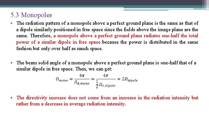
5. 3 Monopoles • The radiation pattern of a monopole above a perfect ground plane is the same as that of a dipole similarly positioned in free space since the fields above the image plane are the same. Therefore, a monopole above a perfect ground plane radiates one-half the total power of a similar dipole in free space because the power is distributed in the same fashion but only over half as much space. • The beam solid angle of a monopole above a perfect ground plane is one-half that of a similar dipole in free space. Then, we can get: • The directivity increase does not come from an increase in the radiation intensity but rather from a decrease in average radiation intensity.

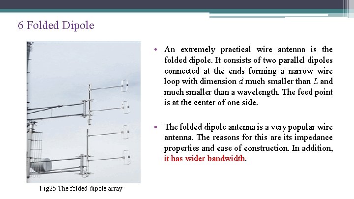
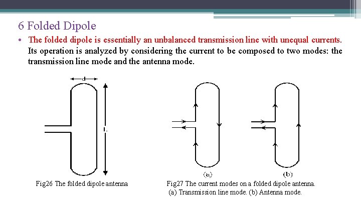
6 Folded Dipole • An extremely practical wire antenna is the folded dipole. It consists of two parallel dipoles connected at the ends forming a narrow wire loop with dimension d much smaller than L and much smaller than a wavelength. The feed point is at the center of one side. • The folded dipole antenna is a very popular wire antenna. The reasons for this are its impedance properties and ease of construction. In addition, it has wider bandwidth. Fig 25 The folded dipole array

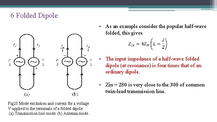
6 Folded Dipole • The folded dipole is essentially an unbalanced transmission line with unequal currents. Its operation is analyzed by considering the current to be composed to two modes: the transmission line mode and the antenna mode. Fig 26 The folded dipole antenna Fig 27 The current modes on a folded dipole antenna. (a) Transmission line mode. (b) Antenna mode.

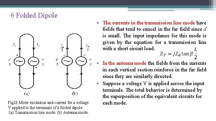
6 Folded Dipole • The currents in the transmission line mode have fields that tend to cancel in the far field since d is small. The input impedance for this mode is given by the equation for a transmission line with a short circuit load. Fig 28 Mode excitation and current for a voltage V applied to the terminals of a folded dipole. (a) Transmission line mode. (b) Antenna mode. • In the antenna mode the fields from the currents in each vertical section reinforce in the far field since they are similarly directed. • Suppose a voltage V is applied across the input terminals. The total behavior is determined by the superposition of the equivalent circuits for each mode.

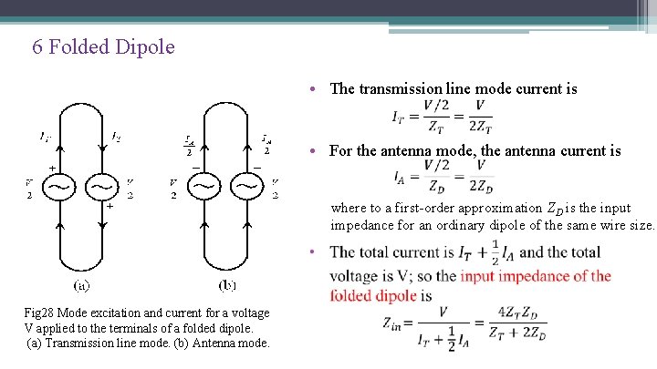
6 Folded Dipole • The transmission line mode current is • For the antenna mode, the antenna current is where to a first-order approximation ZD is the input impedance for an ordinary dipole of the same wire size. Fig 28 Mode excitation and current for a voltage V applied to the terminals of a folded dipole. (a) Transmission line mode. (b) Antenna mode.

6 Folded Dipole • As an example consider the popular half-wave folded, this gives • The input impedance of a half-wave folded dipole (at resonance) is four times that of an ordinary dipole. • Zin = 280 is very close to the 300 of common twin-lead transmission line. Fig 28 Mode excitation and current for a voltage V applied to the terminals of a folded dipole. (a) Transmission line mode. (b) Antenna mode.

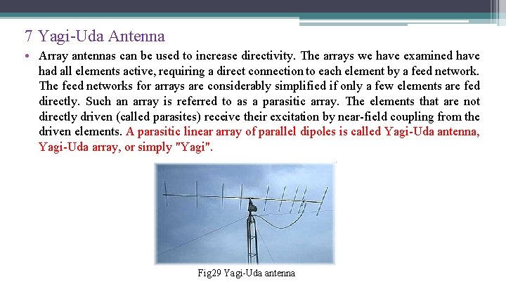
7 Yagi-Uda Antenna • Array antennas can be used to increase directivity. The arrays we have examined have had all elements active, requiring a direct connection to each element by a feed network. The feed networks for arrays are considerably simplified if only a few elements are fed directly. Such an array is referred to as a parasitic array. The elements that are not directly driven (called parasites) receive their excitation by near-field coupling from the driven elements. A parasitic linear array of parallel dipoles is called Yagi-Uda antenna, Yagi-Uda array, or simply "Yagi". Fig 29 Yagi-Uda antenna

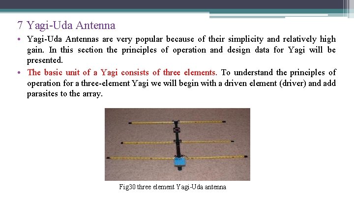
7 Yagi-Uda Antenna • Yagi-Uda Antennas are very popular because of their simplicity and relatively high gain. In this section the principles of operation and design data for Yagi will be presented. • The basic unit of a Yagi consists of three elements. To understand the principles of operation for a three-element Yagi we will begin with a driven element (driver) and add parasites to the array. Fig 30 three element Yagi-Uda antenna

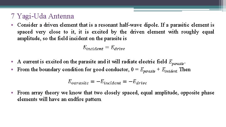
7 Yagi-Uda Antenna • Consider a driven element that is a resonant half-wave dipole. If a parasitic element is spaced very close to it, it is excited by the driven element with roughly equal amplitude, so the field incident on the parasite is • A current is excited on the parasite and it will radiate electric field Eparasite. • From the boundary condition for good conductor, 0 = Eparasite + Eincident. Then • From array theory we know that two closely spaced, equal amplitude, opposite phase elements will have an endfire pattern.

7 Yagi-Uda Antenna • Reflector ▫ The numerical methods demonstrates the general trend of a parasite which is longer than the driver: a single main beam occurs in the endfire direction from the parasite to the driver along the line of the array. Such a parasite is called a reflector because it appears to reflect radiation from the driver. • Director ▫ If the parasite is shorter than the driver, but now placed on the other side of the driver, the pattern effect is similar to that when using a reflector in the sense that main beam enhancement is in the same direction. The parasite is then referred to as a director since it appears to direct radiation in the direction from the driver toward the director.

7 Yagi-Uda Antenna • The single endfire beam created by the use of a reflector or a director alone with a driver suggests that even further enhancement could be achieved with a reflector and a director on opposite sides of a driver. The maximum directivity obtained from a threeelement Yagi is about 9 d. B. • The optimum spacing ( for maximum directivity) are on the order of 0. 15 to 0. 25 wavelength between the reflector and driver and also between the driver to director. Typically the reflector is lengthened 5% or more and the director is shortened 5% or more from the length of resonant length driver.

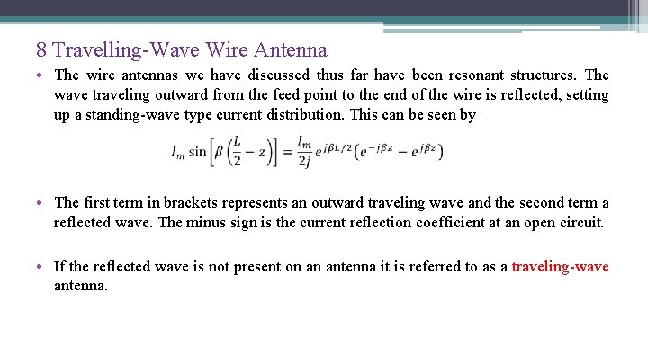
8 Travelling-Wave Wire Antenna • The wire antennas we have discussed thus far have been resonant structures. The wave traveling outward from the feed point to the end of the wire is reflected, setting up a standing-wave type current distribution. This can be seen by • The first term in brackets represents an outward traveling wave and the second term a reflected wave. The minus sign is the current reflection coefficient at an open circuit. • If the reflected wave is not present on an antenna it is referred to as a traveling-wave antenna.

8 Travelling-Wave Wire Antenna Standing wave antennas: • Center-fed linear wire antennas were discussed whose amplitude current distribution was 1. constant for infinitesimal dipoles (l ≤ λ/50) 2. linear (triangular) for short dipoles (λ/50 < l ≤ λ/10) 3. sinusoidal for long dipoles (l > λ/10) • In all cases the phase distribution was assumed to be constant. The sinusoidal current distribution of long open-ended linear antennas is a standing wave constructed by two waves of equal amplitude and 180◦ phase difference at the open end traveling in opposite directions along its length.

8 Travelling-Wave Wire Antenna • The voltage distribution has also a standing wave pattern except that it has maxima (loops) at the end of the line instead of nulls (nodes) as the current. • In each pattern, the maxima and minima repeat every integral number of half wavelengths. There is also a λ/4 spacing between a null and a maximum in each of the wave patterns. • The current and voltage distributions on open-ended wire antennas are similar to the standing wave patterns on open-ended transmission lines. Linear antennas that exhibit current and voltage standing wave patterns formed by reflections from the open end of the wire are referred to as standing wave or resonant antennas.

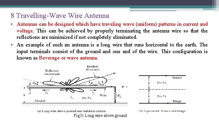
8 Travelling-Wave Wire Antenna • Antennas can be designed which have traveling wave (uniform) patterns in current and voltage. This can be achieved by properly terminating the antenna wire so that the reflections are minimized if not completely eliminated. • An example of such an antenna is a long wire that runs horizontal to the earth. The input terminals consist of the ground and one end of the wire. This configuration is known as Beverage or wave antenna. Fig 31 Long wire above ground

8 Travelling-Wave Wire Antenna • In general, all antennas whose current and voltage distributions can be represented by one or more traveling waves, usually in the same direction, are referred to as traveling wave or nonresonant antennas. A progressive phase pattern is usually associated with the current and voltage distributions. • Standing wave antennas, such as the dipole, can be analyzed as traveling wave antennas with waves propagating in opposite directions (forward and backward) and represented by traveling wave currents If and Ib. • Besides the long wire antenna there are many examples of traveling wave antennas such as dielectric rod (polyrod), helix, and various surface wave antennas. Aperture antennas, such as reflectors and horns, can also be treated as traveling wave antennas. In addition, arrays of closely spaced radiators (usually less than λ/2 apart) can also be analyzed as traveling wave antennas by approximating their current or field distribution by a continuous traveling wave. Yagi-Uda, log-periodic, and slots and holes in a waveguide are some examples of discrete-element traveling wave antennas.

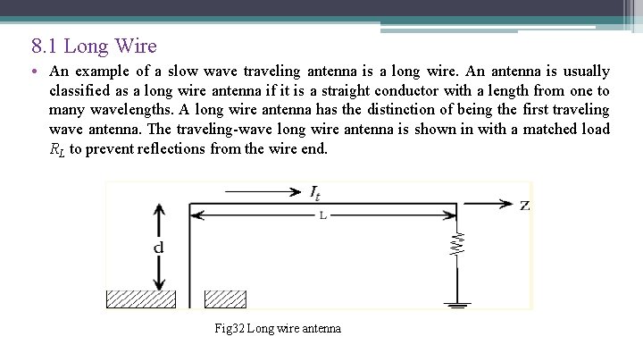
8. 1 Long Wire • An example of a slow wave traveling antenna is a long wire. An antenna is usually classified as a long wire antenna if it is a straight conductor with a length from one to many wavelengths. A long wire antenna has the distinction of being the first traveling wave antenna. The traveling-wave long wire antenna is shown in with a matched load RL to prevent reflections from the wire end. Fig 32 Long wire antenna

8. 1 Long Wire • The height h of the antenna above the ground must be chosen so that the reflected wave (or wave from the image), which includes the phase due to reflection is in phase with the direct wave at the angles of desired maximum radiation. • Simplifying assumptions: ▫ the ground plane effects is ignored and free space; ▫ the details of the feed are assumed to be unimportant, the vertical section of length d is assumed not to radiate; ▫ the radiative and ohmic losses along the wire are small. • Then we can write

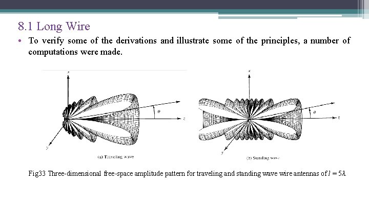
8. 1 Long Wire • To verify some of the derivations and illustrate some of the principles, a number of computations were made. Fig 33 Three-dimensional free-space amplitude pattern for traveling and standing wave wire antennas of l = 5λ.

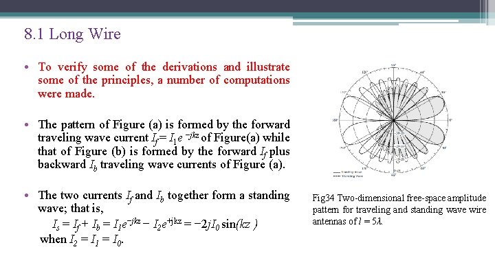
8. 1 Long Wire • To verify some of the derivations and illustrate some of the principles, a number of computations were made. • The pattern of Figure (a) is formed by the forward traveling wave current If = I 1 e −jkz of Figure(a) while that of Figure (b) is formed by the forward If plus backward Ib traveling wave currents of Figure (a). • The two currents If and Ib together form a standing wave; that is, Is = If + Ib = I 1 e−jkz − I 2 e+jkz = − 2 j. I 0 sin(kz ) when I 2 = I 1 = I 0. Fig 34 Two-dimensional free-space amplitude pattern for traveling and standing wave wire antennas of l = 5λ.

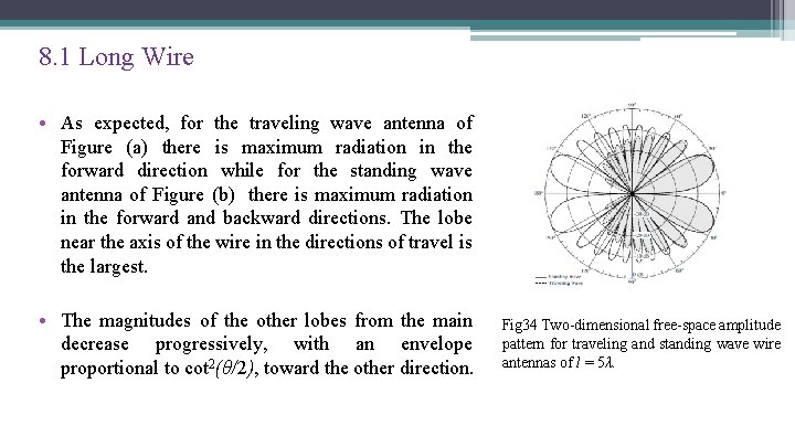
8. 1 Long Wire • As expected, for the traveling wave antenna of Figure (a) there is maximum radiation in the forward direction while for the standing wave antenna of Figure (b) there is maximum radiation in the forward and backward directions. The lobe near the axis of the wire in the directions of travel is the largest. • The magnitudes of the other lobes from the main decrease progressively, with an envelope proportional to cot 2(θ/2), toward the other direction. Fig 34 Two-dimensional free-space amplitude pattern for traveling and standing wave wire antennas of l = 5λ.

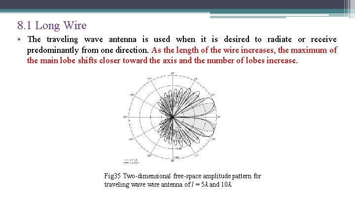
8. 1 Long Wire • The traveling wave antenna is used when it is desired to radiate or receive predominantly from one direction. As the length of the wire increases, the maximum of the main lobe shifts closer toward the axis and the number of lobes increase. Fig 35 Two-dimensional free-space amplitude pattern for traveling wave wire antenna of l = 5λ and 10λ.

8. 1 Long Wire • For traveling wave wire antennas the radiation in the opposite direction from the maximum is suppressed by reducing, if not completely eliminating, the current reflected from the end of the wire. This is accomplished by increasing the diameter of the wire or more successfully by properly terminating it to the ground. • Ideally a complete elimination of the reflections (perfect match) can only be accomplished if the antenna is elevated only at small heights (compared to the wavelength) above the ground, and it is terminated by a resistive load. The value of the load resistor, to achieve the impedance match, is equal to the characteristic impedance of the wire near the ground (which is found using image theory).

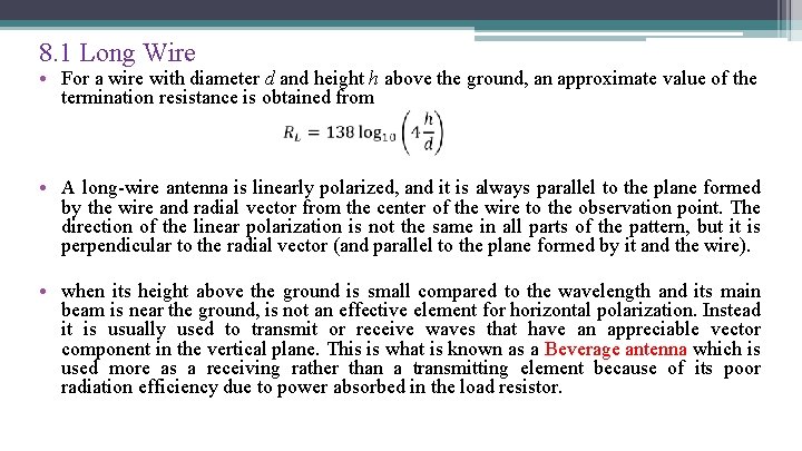
8. 1 Long Wire • For a wire with diameter d and height h above the ground, an approximate value of the termination resistance is obtained from • A long-wire antenna is linearly polarized, and it is always parallel to the plane formed by the wire and radial vector from the center of the wire to the observation point. The direction of the linear polarization is not the same in all parts of the pattern, but it is perpendicular to the radial vector (and parallel to the plane formed by it and the wire). • when its height above the ground is small compared to the wavelength and its main beam is near the ground, is not an effective element for horizontal polarization. Instead it is usually used to transmit or receive waves that have an appreciable vector component in the vertical plane. This is what is known as a Beverage antenna which is used more as a receiving rather than a transmitting element because of its poor radiation efficiency due to power absorbed in the load resistor.

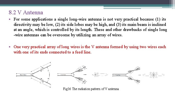
8. 2 V Antenna • For some applications a single long-wire antenna is not very practical because (1) its directivity may be low, (2) its side lobes may be high, and (3) its main beam is inclined at an angle, which is controlled by its length. These and other drawbacks of single long -wire antennas can be overcome by utilizing an array of wires. • One very practical array of long wires is the V antenna formed by using two wires each with one of its ends connected to a feed line. Fig 36 The radiation pattern of V antenna

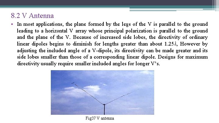
8. 2 V Antenna • In most applications, the plane formed by the legs of the V is parallel to the ground leading to a horizontal V array whose principal polarization is parallel to the ground and the plane of the V. Because of increased side lobes, the directivity of ordinary linear dipoles begins to diminish for lengths greater than about 1. 25λ, However by adjusting the included angle of a V-dipole, its directivity can be made greater and its side lobes smaller than those of a corresponding linear dipole. Designs for maximum directivity usually require smaller included angles for longer V’s. Fig 37 V antenna

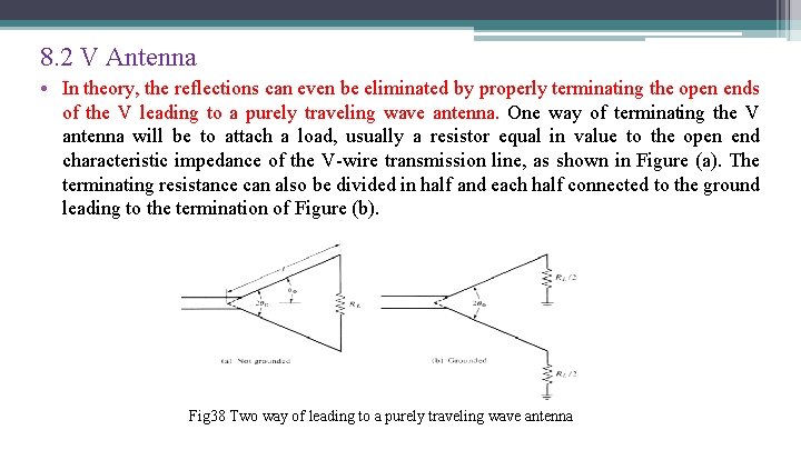
8. 2 V Antenna • In theory, the reflections can even be eliminated by properly terminating the open ends of the V leading to a purely traveling wave antenna. One way of terminating the V antenna will be to attach a load, usually a resistor equal in value to the open end characteristic impedance of the V-wire transmission line, as shown in Figure (a). The terminating resistance can also be divided in half and each half connected to the ground leading to the termination of Figure (b). Fig 38 Two way of leading to a purely traveling wave antenna

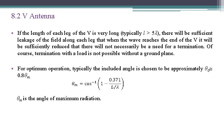
8. 2 V Antenna • If the length of each leg of the V is very long (typically l > 5λ), there will be sufficient leakage of the field along each leg that when the wave reaches the end of the V it will be sufficiently reduced that there will not necessarily be a need for a termination. Of course, termination with a load is not possible without a ground plane. • For optimum operation, typically the included angle is chosen to be approximately θ 0 0. 8θm. θm is the angle of maximum radiation.

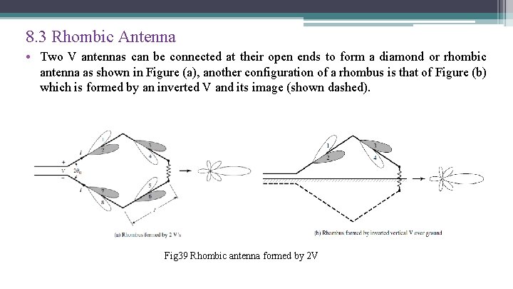
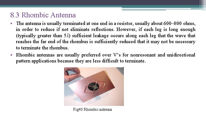
8. 3 Rhombic Antenna • Two V antennas can be connected at their open ends to form a diamond or rhombic antenna as shown in Figure (a), another configuration of a rhombus is that of Figure (b) which is formed by an inverted V and its image (shown dashed). Fig 39 Rhombic antenna formed by 2 V

8. 3 Rhombic Antenna • The antenna is usually terminated at one end in a resistor, usually about 600– 800 ohms, in order to reduce if not eliminate reflections. However, if each leg is long enough (typically greater than 5λ) sufficient leakage occurs along each leg that the wave that reaches the far end of the rhombus is sufficiently reduced that it may not be necessary to terminate the rhombus. • Rhombic antennas are usually preferred over V’s for nonresonant and unidirectional pattern applications because they are less difficult to terminate. Fig 40 Rhombic antenna

66 Homework: • A resonant center-fed dipole is connected to a 50 -ohm line. It is desired to maintain the input VSWR = 2. (a) What should the largest input resistance of the dipole be to maintain the VSWR = 2? (b) What should the length (in wavelengths) of the dipole be to meet the specification? (c) What is the radiation resistance of the dipole? • Group discussion and write a report in teamwork: Conclude the similarity and difference between each wire antenna

Thank you!