Anisotropic Gaussian Mutations for Metropolis Light Transport through

Anisotropic Gaussian Mutations for Metropolis Light Transport through Hessian-Hamiltonian Dynamics Tzu-Mao Li 1 Jaakko Lehtinen 2, 3 Ravi Ramamoorthi 4 Wenzel Jakob 5 Frédo Durand 1 1 MIT 2 Aalto University 3 NVIDIA CSAIL 4 UC San Diego 5 ETH Zürich

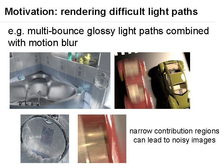
Motivation: rendering difficult light paths e. g. multi-bounce glossy light paths combined with motion blur narrow contribution regions can lead to noisy images

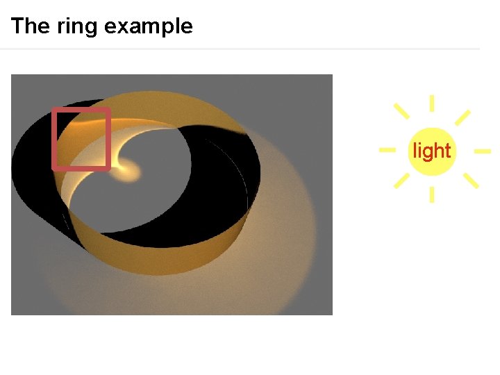
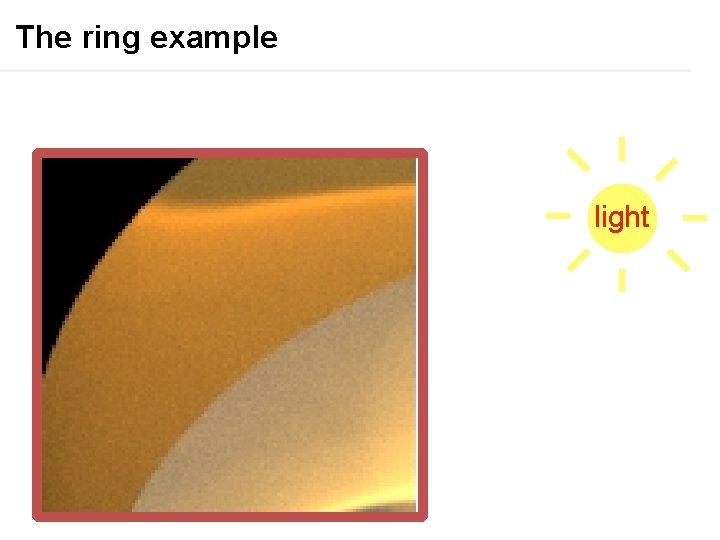
The ring example light

The ring example light

The ring example light

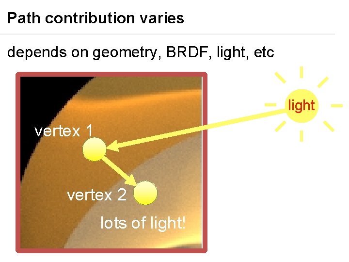
Path contribution varies depends on geometry, BRDF, light, etc light vertex 1 vertex 2 lots of light!

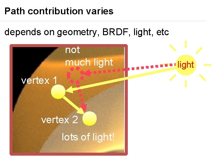
Path contribution varies depends on geometry, BRDF, light, etc not much light vertex 1 vertex 2 lots of light! light

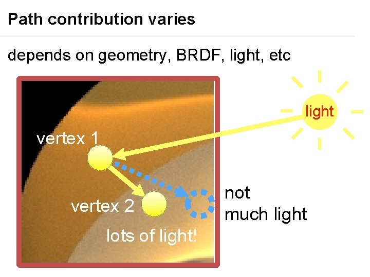
Path contribution varies depends on geometry, BRDF, light, etc light vertex 1 vertex 2 lots of light! not much light

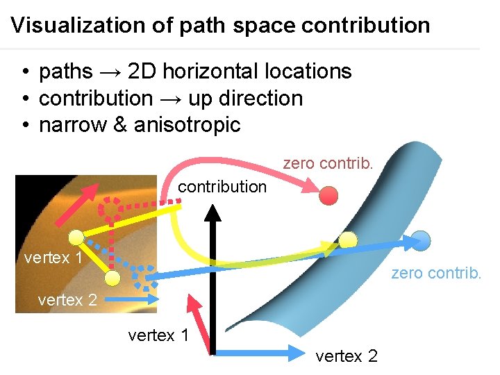
Visualization of path space contribution • paths → 2 D horizontal locations • contribution → up direction • narrow & anisotropic zero contribution vertex 1 zero contrib. vertex 2 vertex 1 vertex 2

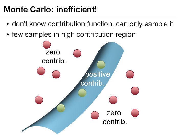
Monte Carlo: inefficient! • don’t know contribution function, can only sample it • few samples in high contribution region zero contrib. positive contrib. zero contrib.

Metropolis Light Transport [Veach 1997] idea: stays in high contribution region with Markov chain sample n+2 sample n+1

Metropolis Light Transport [Veach 1997] idea: stays in high contribution region with Markov chain sample n+1 drawn from proposal distribution sample n+1 proposal distribution

Metropolis Light Transport [Veach 1997] problem: proposals with low contribution are probabilistically rejected rejected

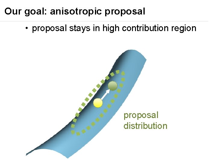
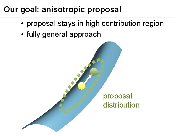
Our goal: anisotropic proposal • proposal stays in high contribution region proposal distribution

Previous work [Jakob 2012, Kaplanyan 2014] • specialized for microfacet BRDF & mirror directions • proposal in special directions

Our goal: anisotropic proposal • proposal stays in high contribution region • fully general approach proposal distribution

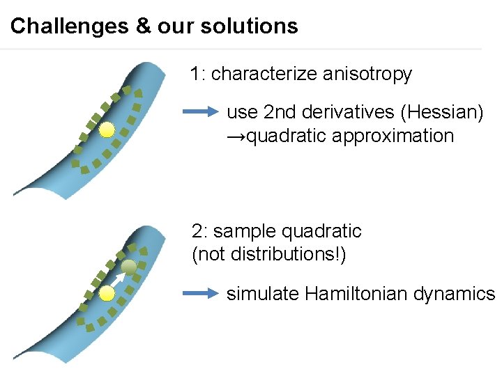
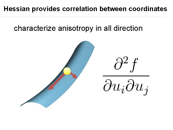
Challenges & our solutions 1: characterize anisotropy use 2 nd derivatives (Hessian) →quadratic approximation 2: sample quadratic (not distributions!) simulate Hamiltonian dynamics

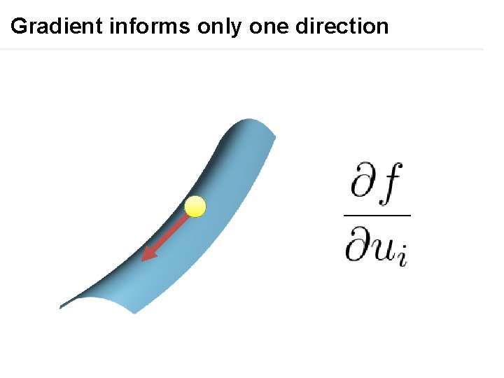
Gradient informs only one direction

Hessian provides correlation between coordinates characterize anisotropy in all direction

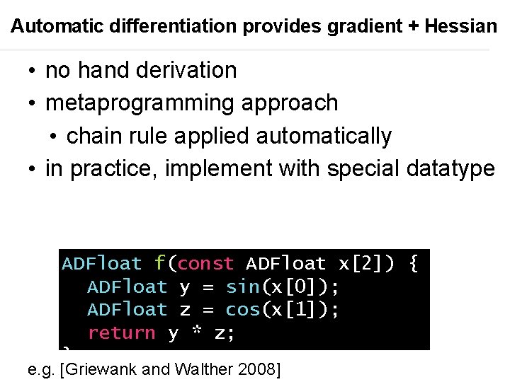
Automatic differentiation provides gradient + Hessian • no hand derivation • metaprogramming approach • chain rule applied automatically • in practice, implement with special datatype ADFloat f(const ADFloat x[2]) { ADFloat y = sin(x[0]); ADFloat z = cos(x[1]); return y * z; } e. g. [Griewank and Walther 2008]

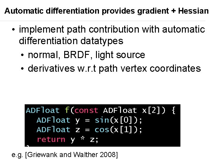
Automatic differentiation provides gradient + Hessian • implement path contribution with automatic differentiation datatypes • normal, BRDF, light source • derivatives w. r. t path vertex coordinates ADFloat f(const ADFloat x[2]) { ADFloat y = sin(x[0]); ADFloat z = cos(x[1]); return y * z; } e. g. [Griewank and Walther 2008]

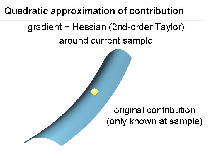
Quadratic approximation of contribution gradient + Hessian (2 nd-order Taylor) around current sample original contribution (only known at sample)

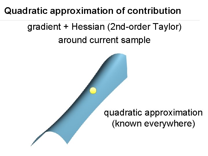
Quadratic approximation of contribution gradient + Hessian (2 nd-order Taylor) around current sample quadratic approximation (known everywhere)

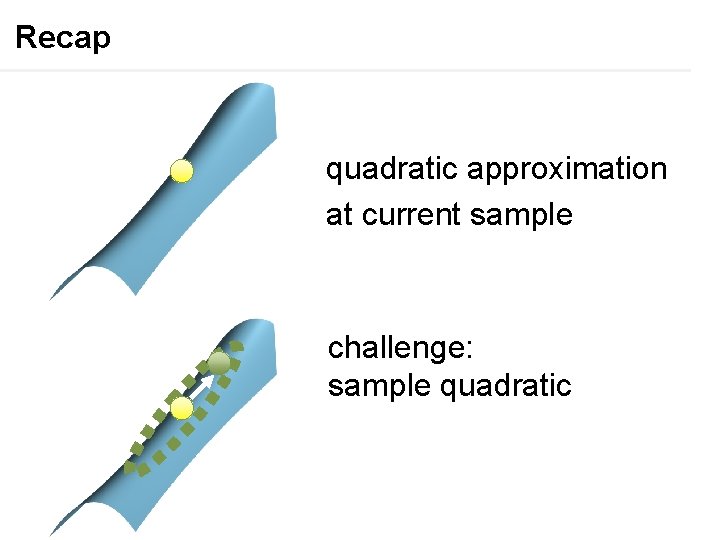
Recap quadratic approximation at current sample challenge: sample quadratic

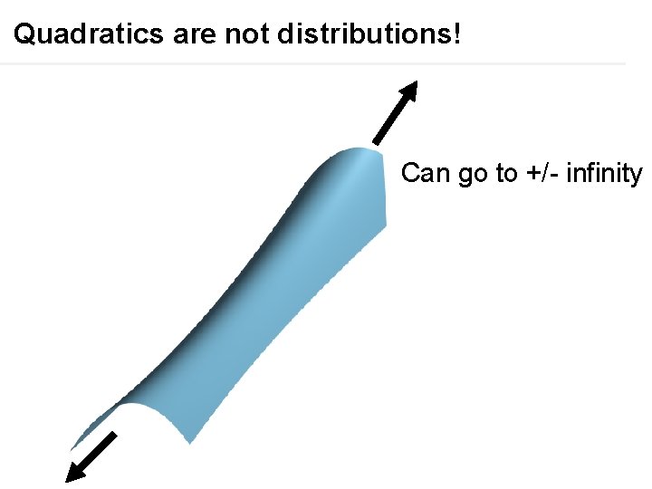
Quadratics are not distributions! Can go to +/- infinity

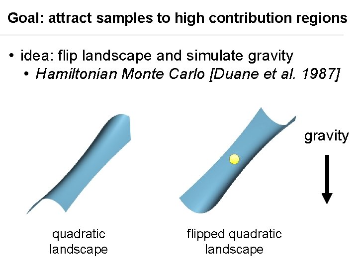
Goal: attract samples to high contribution regions • idea: flip landscape and simulate gravity • Hamiltonian Monte Carlo [Duane et al. 1987] gravity quadratic landscape flipped quadratic landscape

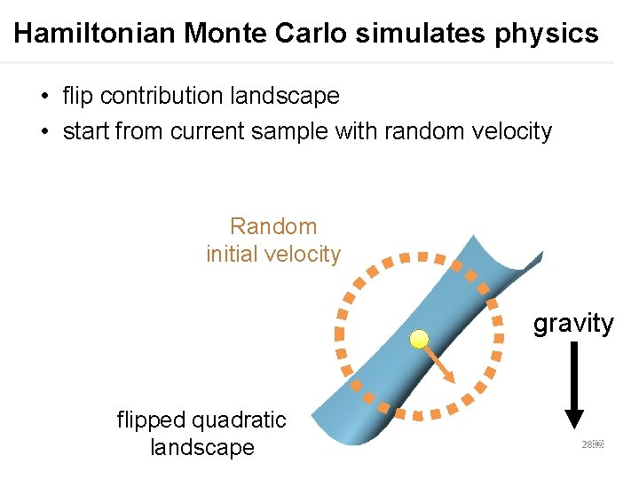
Hamiltonian Monte Carlo simulates physics • flip contribution landscape • start from current sample with random velocity Random initial velocity gravity flipped quadratic landscape 28

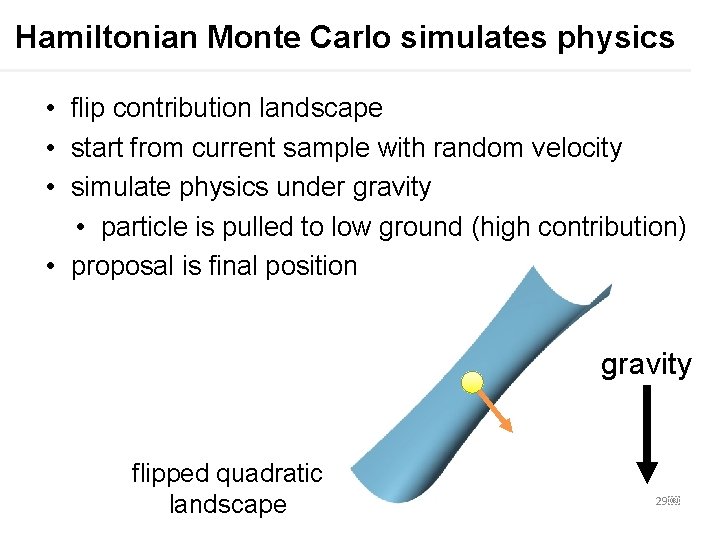
Hamiltonian Monte Carlo simulates physics • flip contribution landscape • start from current sample with random velocity • simulate physics under gravity • particle is pulled to low ground (high contribution) • proposal is final position gravity flipped quadratic landscape 29

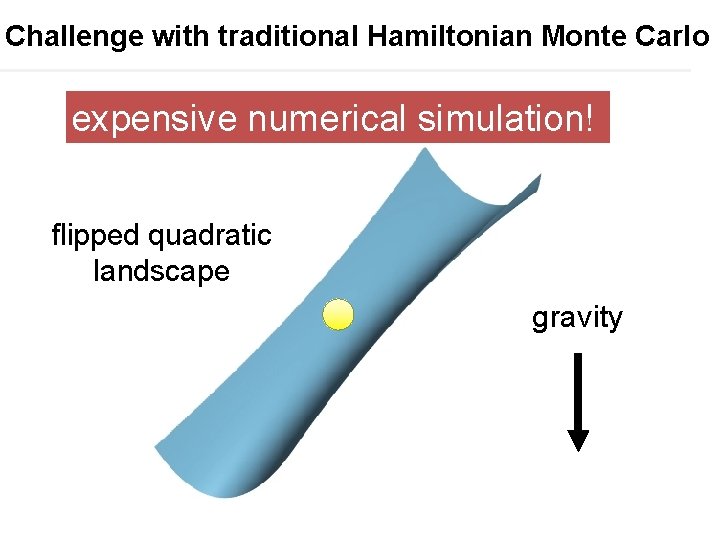
Challenge with traditional Hamiltonian Monte Carlo expensive numerical simulation! flipped quadratic landscape gravity

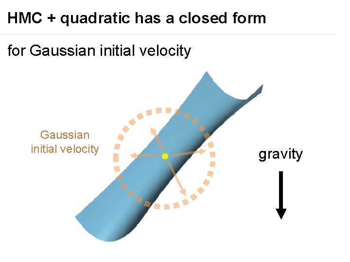
HMC + quadratic has a closed form for Gaussian initial velocity gravity

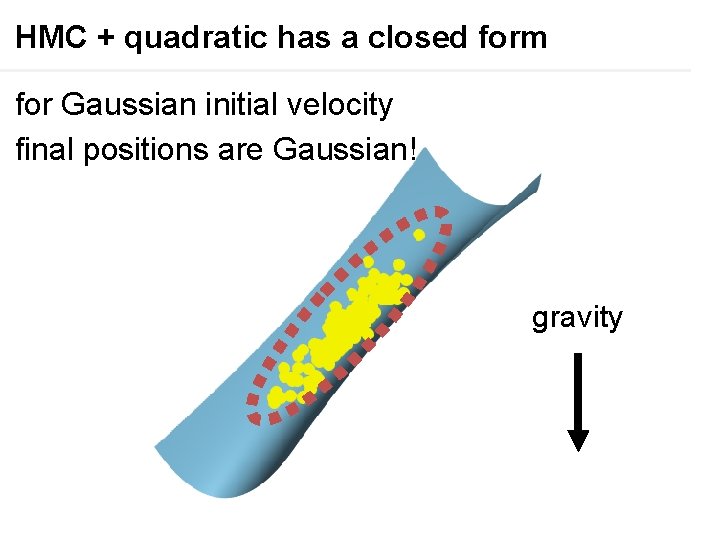
HMC + quadratic has a closed form for Gaussian initial velocity final positions are Gaussian! gravity

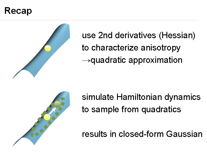
Recap use 2 nd derivatives (Hessian) to characterize anisotropy →quadratic approximation simulate Hamiltonian dynamics to sample from quadratics results in closed-form Gaussian

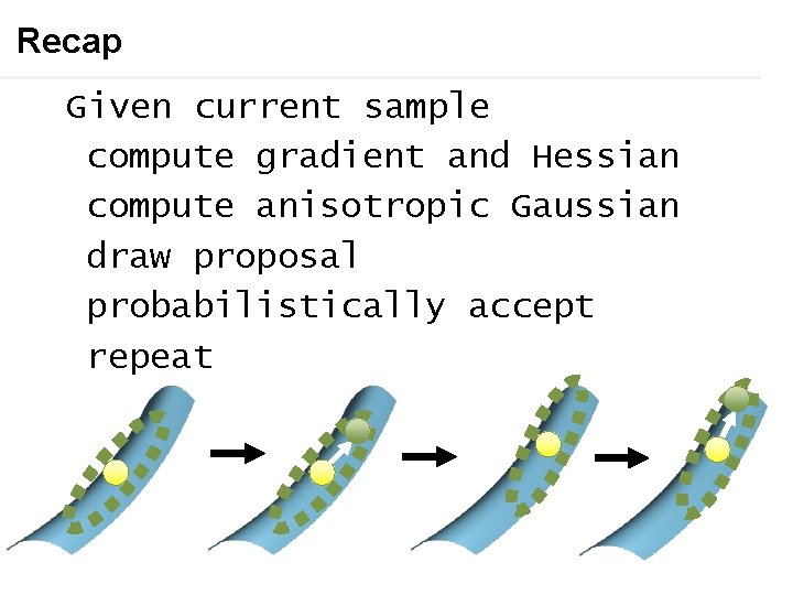
Recap Given current sample compute gradient and Hessian compute anisotropic Gaussian draw proposal probabilistically accept repeat

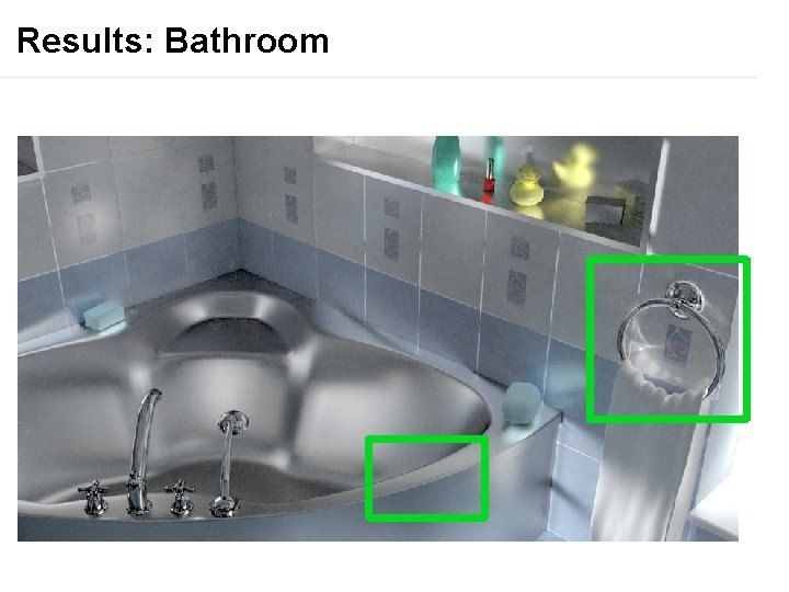
Results: Bathroom

Bathroom: equal-time (10 mins) comparisons MMLT [Hachisuka 2014] MEMLT [Jakob 2012] OURS Reference (2 days) HSLT [Kaplanyan 2014, Hanika 2015]

Bathroom: equal-time (10 mins) comparisons MMLT [Hachisuka 2014] MEMLT [Jakob 2012] OURS Reference (2 days) HSLT [Kaplanyan 2014, Hanika 2015]

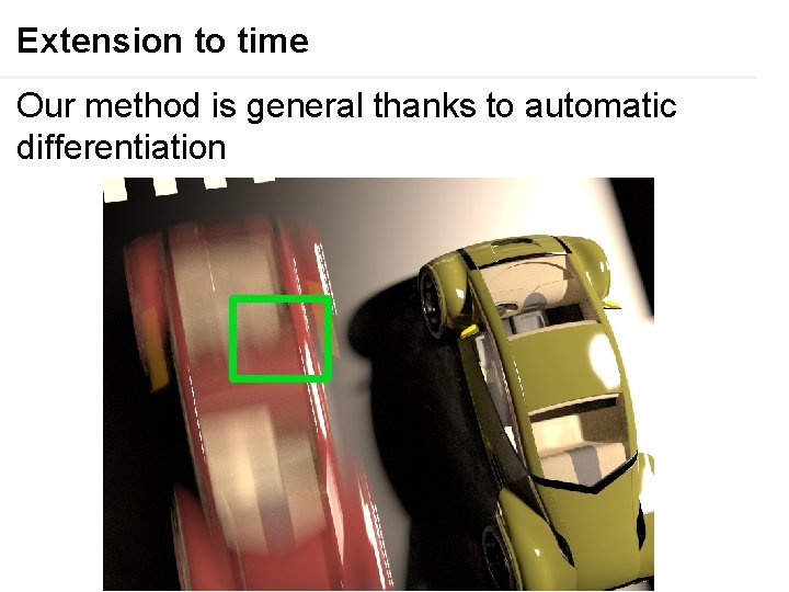
Extension to time Our method is general thanks to automatic differentiation

Cars: equal-time (20 mins) comparisons MMLT [Hachisuka 2014] MEMLT [Jakob 2012] OURS Reference (12 hours)

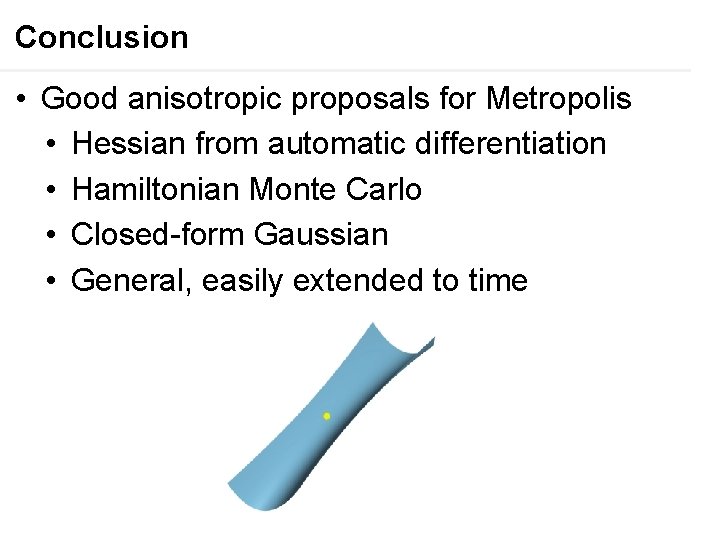
Conclusion • Good anisotropic proposals for Metropolis • Hessian from automatic differentiation • Hamiltonian Monte Carlo • Closed-form Gaussian • General, easily extended to time