Agenda Warm Up min Checkup time Homework AP

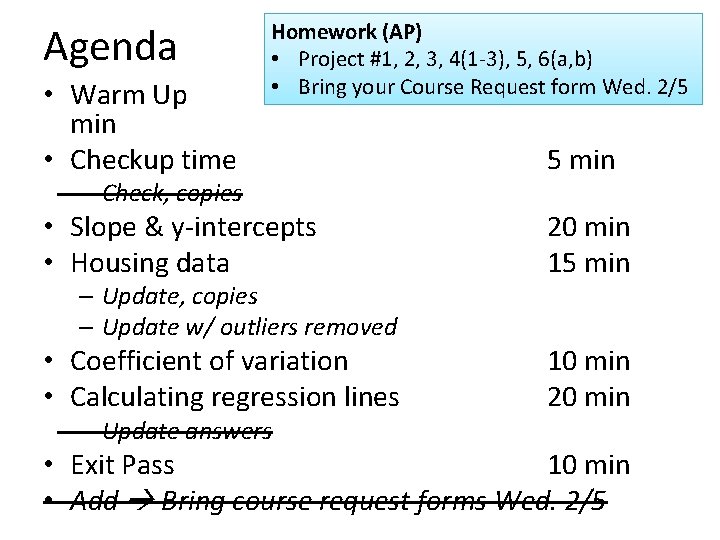
Agenda • Warm Up min • Checkup time Homework (AP) • Project #1, 2, 3, 4(1 -3), 5, 6(a, b) • Bring your Course Request form Wed. 10 2/5 – Check, copies 5 min • Slope & y-intercepts • Housing data 20 min 15 min • Coefficient of variation • Calculating regression lines 10 min 20 min – Update, copies – Update w/ outliers removed – Update answers • Exit Pass 10 min • Add Bring course request forms Wed. 2/5

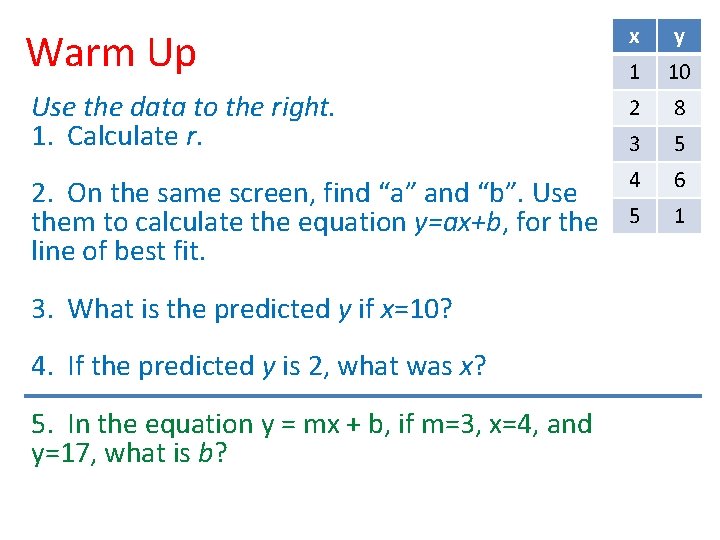
x y 1 10 Use the data to the right. 1. Calculate r. 2 8 3 5 2. On the same screen, find “a” and “b”. Use them to calculate the equation y=ax+b, for the line of best fit. 4 6 5 1 Warm Up 3. What is the predicted y if x=10? 4. If the predicted y is 2, what was x? 5. In the equation y = mx + b, if m=3, x=4, and y=17, what is b?

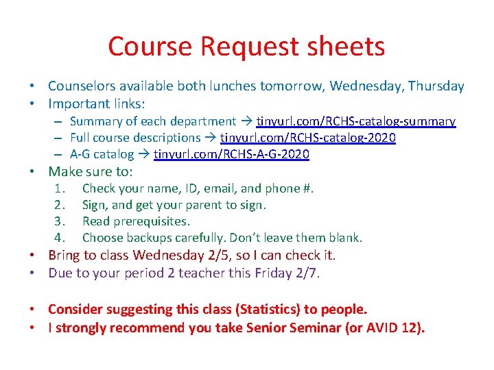
Course Request sheets • Counselors available both lunches tomorrow, Wednesday, Thursday • Important links: – Summary of each department tinyurl. com/RCHS-catalog-summary – Full course descriptions tinyurl. com/RCHS-catalog-2020 – A-G catalog tinyurl. com/RCHS-A-G-2020 • Make sure to: 1. 2. 3. 4. Check your name, ID, email, and phone #. Sign, and get your parent to sign. Read prerequisites. Choose backups carefully. Don’t leave them blank. • Bring to class Wednesday 2/5, so I can check it. • Due to your period 2 teacher this Friday 2/7. • Consider suggesting this class (Statistics) to people. • I strongly recommend you take Senior Seminar (or AVID 12).

Checkup

• Goodbye Einstein. Dead. Murdered.

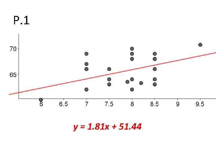
P. 1 y = 1. 81 x + 51. 44

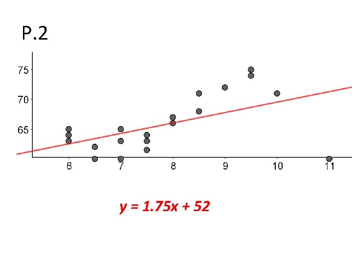
P. 2 y = 1. 75 x + 52

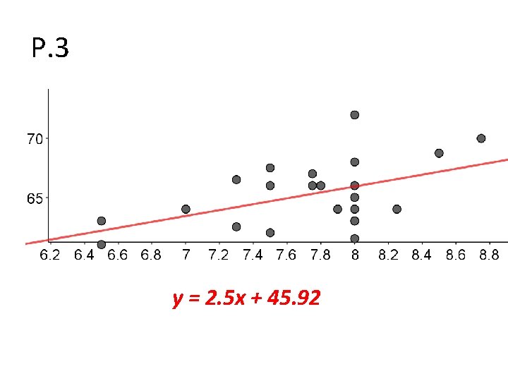
P. 3 y = 2. 5 x + 45. 92

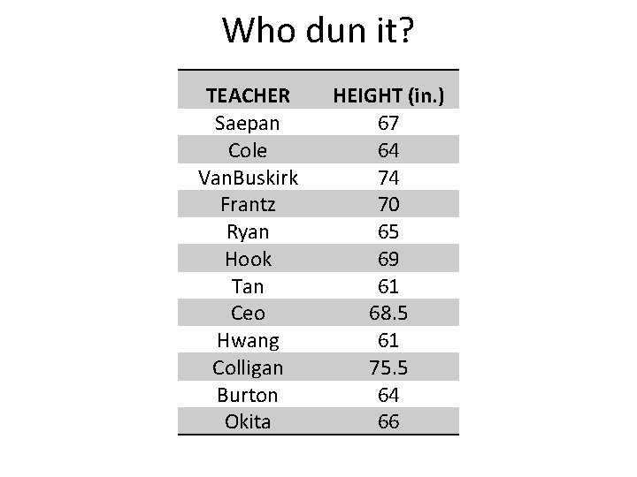
Who dun it? TEACHER Saepan Cole Van. Buskirk Frantz Ryan Hook Tan Ceo Hwang Colligan Burton Okita HEIGHT (in. ) 67 64 74 70 65 69 61 68. 5 61 75. 5 64 66

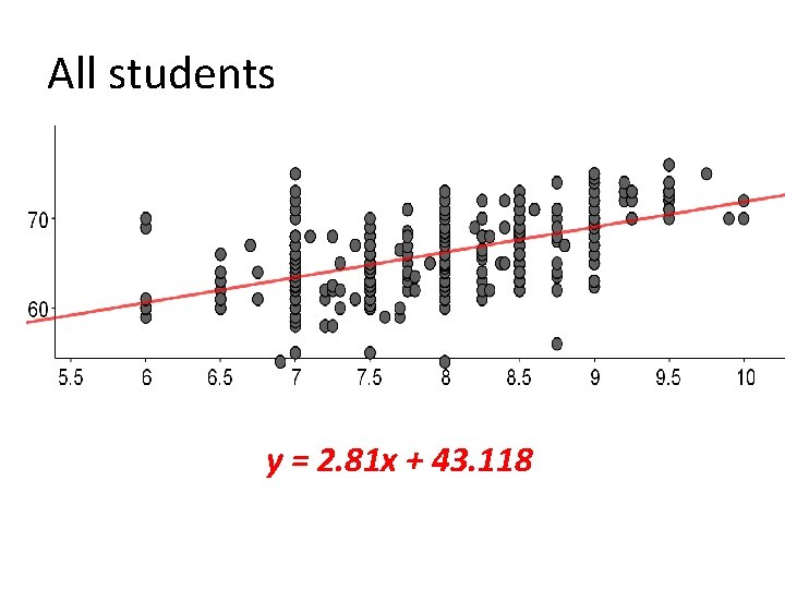
All students y = 2. 81 x + 43. 118

Who dun it? TEACHER Saepan Cole Van. Buskirk Frantz Ryan Hook Tan Ceo Hwang Colligan Burton Okita HEIGHT (in. ) 67 64 74 70 65 69 61 68. 5 61 75. 5 64 66

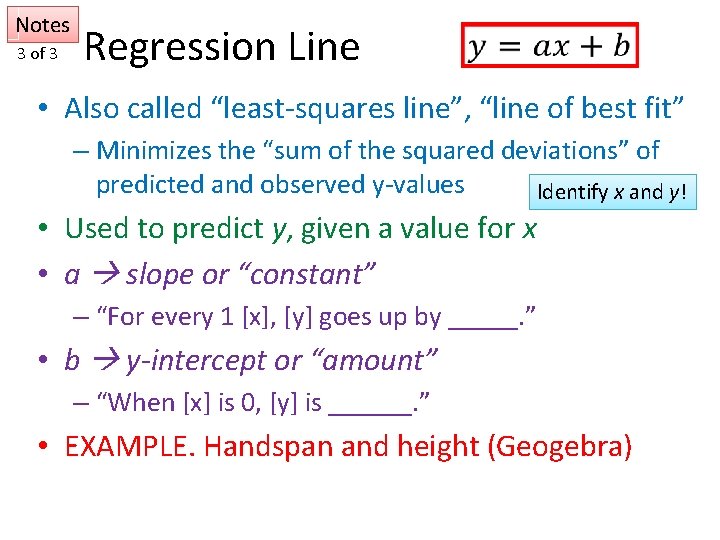
Notes 3 of 3 Regression Line • Also called “least-squares line”, “line of best fit” – Minimizes the “sum of the squared deviations” of predicted and observed y-values Identify x and y! • Used to predict y, given a value for x • a slope or “constant” – “For every 1 [x], [y] goes up by _____. ” • b y-intercept or “amount” – “When [x] is 0, [y] is ______. ” • EXAMPLE. Handspan and height (Geogebra)

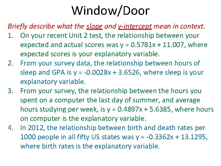
Window/Door Briefly describe what the slope and y-intercept mean in context. 1. On your recent Unit 2 test, the relationship between your expected and actual scores was y = 0. 5781 x + 11. 007, where expected scores is your explanatory variable. 2. From your survey data, the relationship between hours of sleep and GPA is y = -0. 0028 x + 3. 6526, where sleep is your explanatory variable. 3. From your survey, the relationship between the hours you spent on a computer the last day of summer, and average hours studying per week, is y = 0. 4897 x + 5. 6385, where hours on computer is the explanatory variable. 4. In 2012, the relationship between birth and death rates per 1000 people in all fifty US states was y = -0. 3362 x + 13. 1295, where birth rates is the explanatory variable.

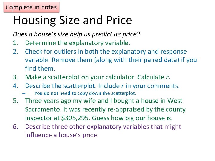
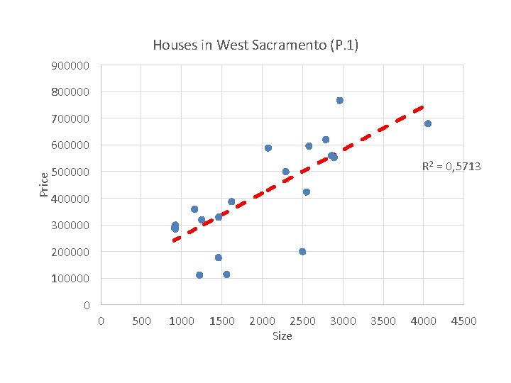
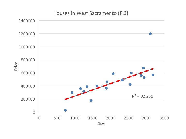
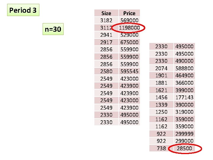
Complete in notes Housing Size and Price Does a house’s size help us predict its price? 1. Determine the explanatory variable. 2. Check for outliers in both the explanatory and response variable. Remove them (along with their paired data) if you find them. 3. Make a scatterplot on your calculator. Calculate r. 4. Describe the scatterplot. Include r in your comments. – You do not need to copy down the scatterplot. 5. Three years ago my wife and I bought a house in West Sacramento. It was recently re-appraised by the county inspector at $305, 295. Guess how big our house is. 6. Describe three other explanatory variables that might influence a house’s price.

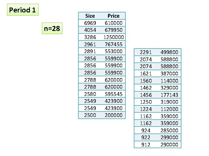
Period 1 n=28 Size 6969 4054 3286 2961 2891 2856 2788 2580 2549 2500 Price 610000 679950 1250000 767455 553000 559900 620000 595545 423900 200000 2291 2074 1621 1560 1462 1456 1250 1224 1162 924 922 912 499800 588800 387000 114000 329000 177143 319000 112000 359000 285000 299000 290000

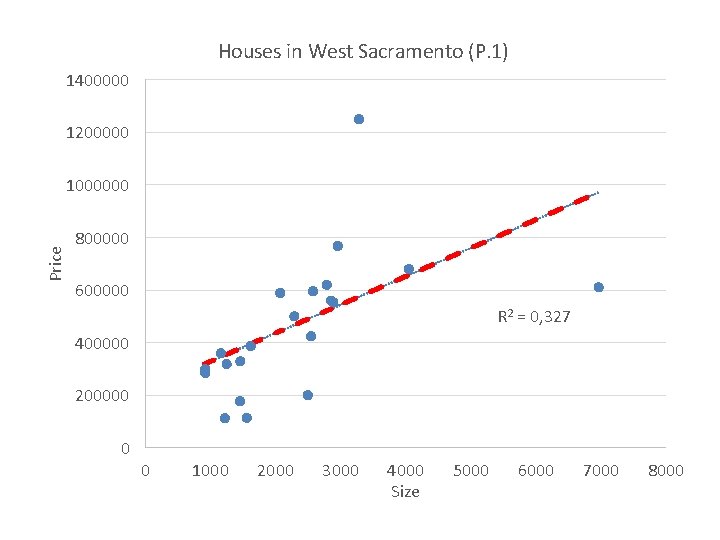
Houses in West Sacramento (P. 1) 1400000 1200000 Price 1000000 800000 600000 R 2 = 0, 327 400000 200000 0 0 1000 2000 3000 4000 Size 5000 6000 7000 8000

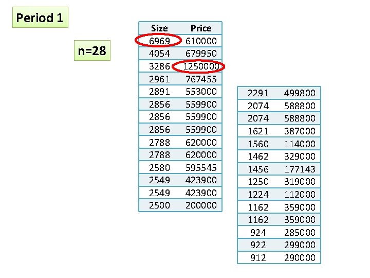
Period 1 n=28 Size 6969 4054 3286 2961 2891 2856 2788 2580 2549 2500 Price 610000 679950 1250000 767455 553000 559900 620000 595545 423900 200000 2291 2074 1621 1560 1462 1456 1250 1224 1162 924 922 912 499800 588800 387000 114000 329000 177143 319000 112000 359000 285000 299000 290000

Houses in West Sacramento (P. 1) 900000 800000 700000 Price 600000 R 2 = 0, 5713 500000 400000 300000 200000 100000 0 0 500 1000 1500 2000 2500 Size 3000 3500 4000 4500

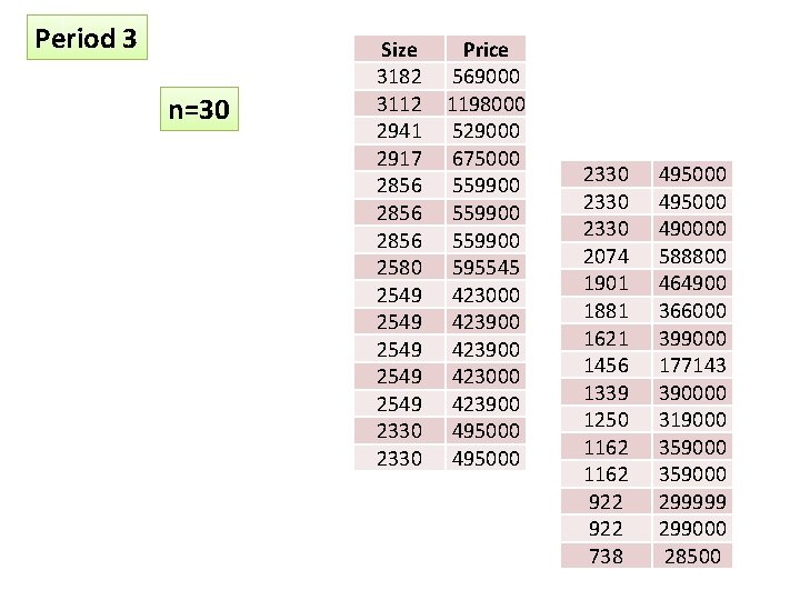
Period 3 n=30 Size 3182 3112 2941 2917 2856 2580 2549 2549 2330 Price 569000 1198000 529000 675000 559900 595545 423000 423900 495000 2330 2074 1901 1881 1621 1456 1339 1250 1162 922 738 495000 490000 588800 464900 366000 399000 177143 390000 319000 359000 299999 299000 28500

Houses in West Sacramento (P. 3) 1400000 1200000 Price 1000000 800000 600000 400000 R 2 = 0, 5231 200000 0 0 500 1000 1500 Size 2000 2500 3000 3500

Period 3 n=30 Size 3182 3112 2941 2917 2856 2580 2549 2549 2330 Price 569000 1198000 529000 675000 559900 595545 423000 423900 495000 2330 2074 1901 1881 1621 1456 1339 1250 1162 922 738 495000 490000 588800 464900 366000 399000 177143 390000 319000 359000 299999 299000 28500

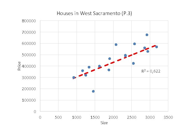
Houses in West Sacramento (P. 3) 800000 700000 600000 Price 500000 400000 R 2 = 0, 622 300000 200000 100000 0 0 500 1000 1500 Size 2000 2500 3000 3500

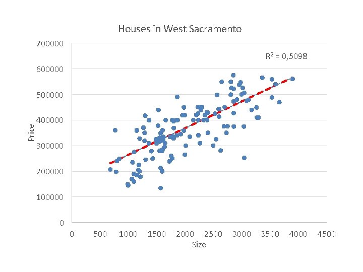
Houses in West Sacramento 700000 R 2 = 0, 5098 600000 Price 500000 400000 300000 200000 100000 0 0 500 1000 1500 2000 2500 Size 3000 3500 4000 4500

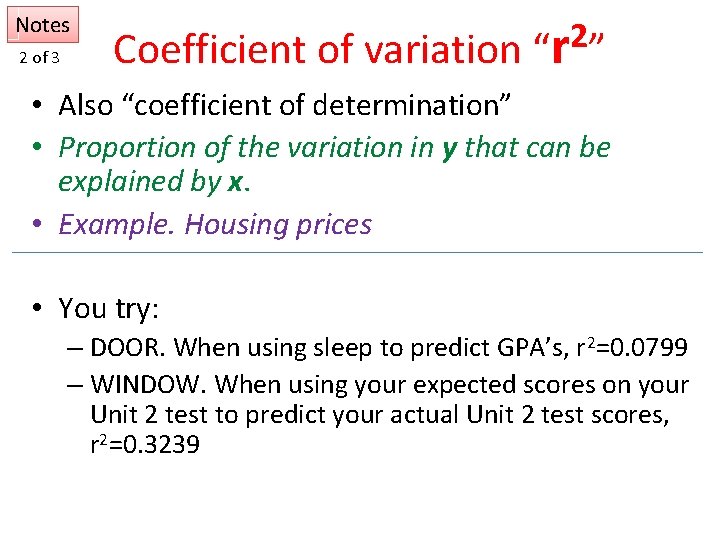
Notes 2 of 3 2 Coefficient of variation “r ” • Also “coefficient of determination” • Proportion of the variation in y that can be explained by x. • Example. Housing prices • You try: – DOOR. When using sleep to predict GPA’s, r 2=0. 0799 – WINDOW. When using your expected scores on your Unit 2 test to predict your actual Unit 2 test scores, r 2=0. 3239

Equation from slope and 1 point • Warm Up #5 5. In the equation y = mx + b, if m=3, x=4, and y=17, what is b?

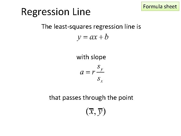
Regression Line The least-squares regression line is with slope that passes through the point Formula sheet

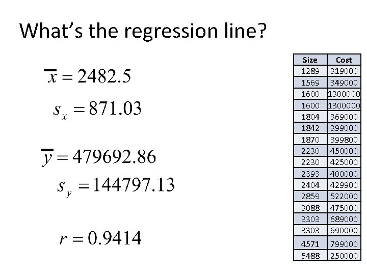
What’s the regression line? Size Cost 1289 319000 1569 349000 1600 1300000 1804 369000 1842 399000 1870 399800 2230 450000 2230 425000 2393 400000 2404 429900 2859 522000 3088 475000 3303 689000 3303 690000 4571 5488 799000 250000

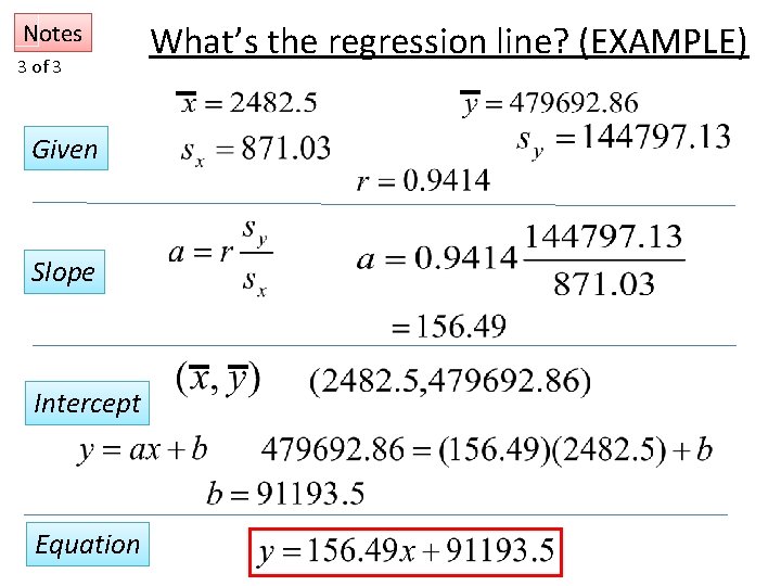
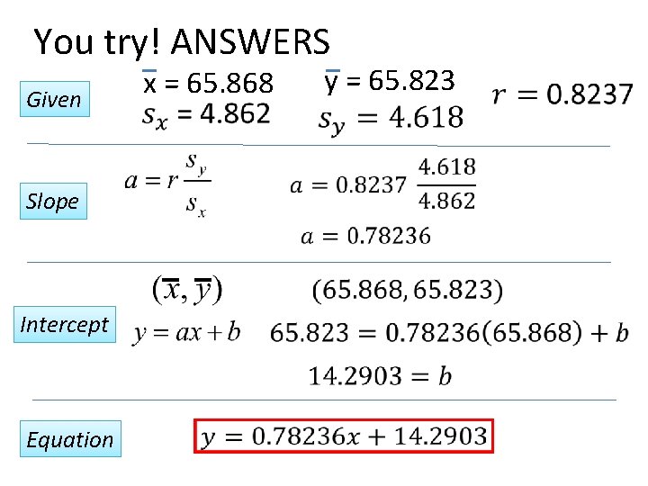
Notes 3 of 3 Given Slope Intercept Equation What’s the regression line? (EXAMPLE)

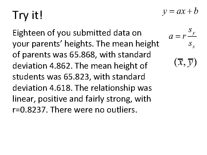
Try it! Eighteen of you submitted data on your parents’ heights. The mean height of parents was 65. 868, with standard deviation 4. 862. The mean height of students was 65. 823, with standard deviation 4. 618. The relationship was linear, positive and fairly strong, with r=0. 8237. There were no outliers.

You try! ANSWERS Given Slope Intercept Equation x = 65. 868 y = 65. 823

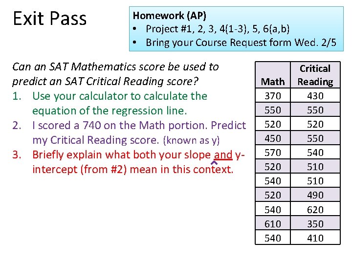
Exit Pass Homework (AP) • Project #1, 2, 3, 4(1 -3), 5, 6(a, b) • Bring your Course Request form Wed. 2/5 Can an SAT Mathematics score be used to predict an SAT Critical Reading score? 1. Use your calculator to calculate the equation of the regression line. 2. I scored a 740 on the Math portion. Predict my Critical Reading score. (known as y) 3. Briefly explain what both your slope and yintercept (from #2) mean in this context. Math 370 550 520 450 570 520 540 610 540 Critical Reading 430 550 520 550 540 510 490 620 350 410