A Sex Determination 1 Environmental Sex Determination 2

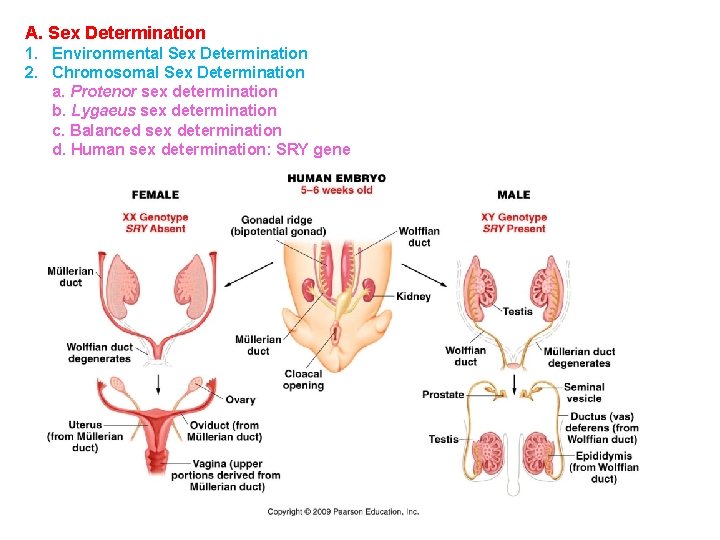
A. Sex Determination 1. Environmental Sex Determination 2. Chromosomal Sex Determination a. Protenor sex determination b. Lygaeus sex determination c. Balanced sex determination d. Human sex determination: SRY gene

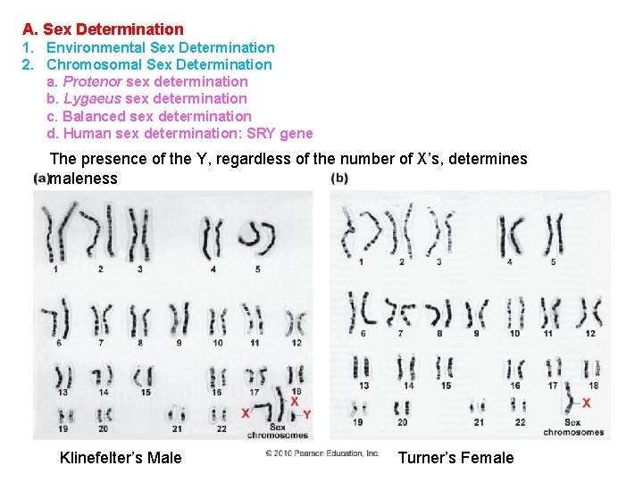
A. Sex Determination 1. Environmental Sex Determination 2. Chromosomal Sex Determination a. Protenor sex determination b. Lygaeus sex determination c. Balanced sex determination d. Human sex determination: SRY gene The presence of the Y, regardless of the number of X’s, determines maleness Klinefelter’s Male Turner’s Female

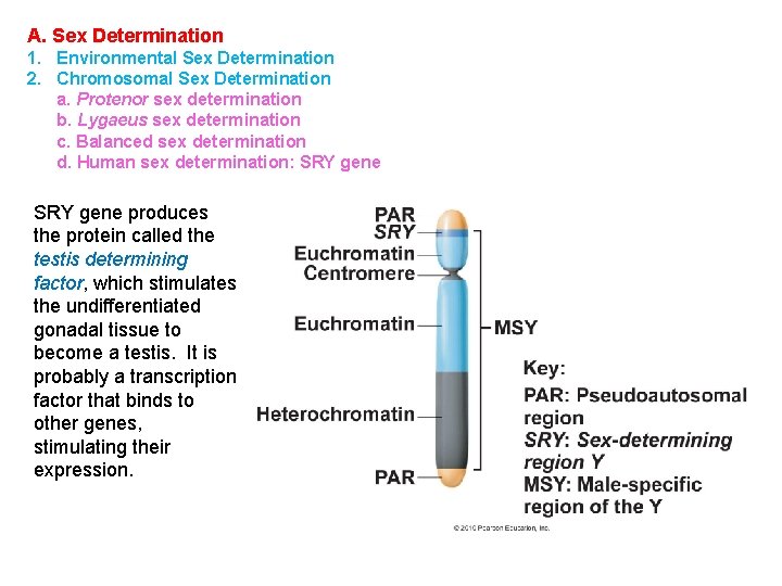
A. Sex Determination 1. Environmental Sex Determination 2. Chromosomal Sex Determination a. Protenor sex determination b. Lygaeus sex determination c. Balanced sex determination d. Human sex determination: SRY gene produces the protein called the testis determining factor, which stimulates the undifferentiated gonadal tissue to become a testis. It is probably a transcription factor that binds to other genes, stimulating their expression.

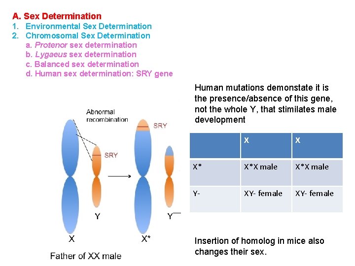
A. Sex Determination 1. Environmental Sex Determination 2. Chromosomal Sex Determination a. Protenor sex determination b. Lygaeus sex determination c. Balanced sex determination d. Human sex determination: SRY gene Human mutations demonstate it is the presence/absence of this gene, not the whole Y, that stimilates male development X X X* X*X male Y- XY- female Insertion of homolog in mice also changes their sex.

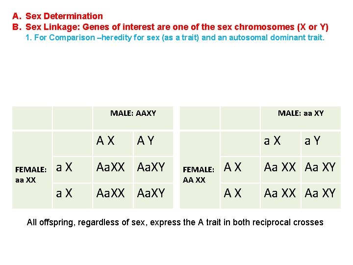
A. Sex Determination B. Sex Linkage: Genes of interest are one of the sex chromosomes (X or Y) 1. For Comparison –heredity for sex (as a trait) and an autosomal dominant trait. MALE: AAXY AX FEMALE: aa XX MALE: aa XY AY a. X Aa. XX Aa. XY a. X FEMALE: AA XX a. Y AX Aa XX Aa XY All offspring, regardless of sex, express the A trait in both reciprocal crosses

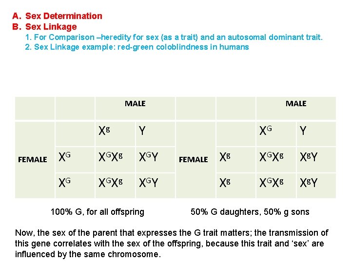
A. Sex Determination B. Sex Linkage 1. For Comparison –heredity for sex (as a trait) and an autosomal dominant trait. 2. Sex Linkage example: red-green coloblindness in humans MALE FEMALE Xg Y XG XG Xg XG Y 100% G, for all offspring MALE FEMALE XG Y Xg XG Xg Xg Y 50% G daughters, 50% g sons Now, the sex of the parent that expresses the G trait matters; the transmission of this gene correlates with the sex of the offspring, because this trait and ‘sex’ are influenced by the same chromosome.

A. Sex Determination B. Sex Linkage 1. For Comparison –heredity for sex (as a trait) and an autosomal dominant trait. 2. Sex Linkage example: red-green coloblindness in humans

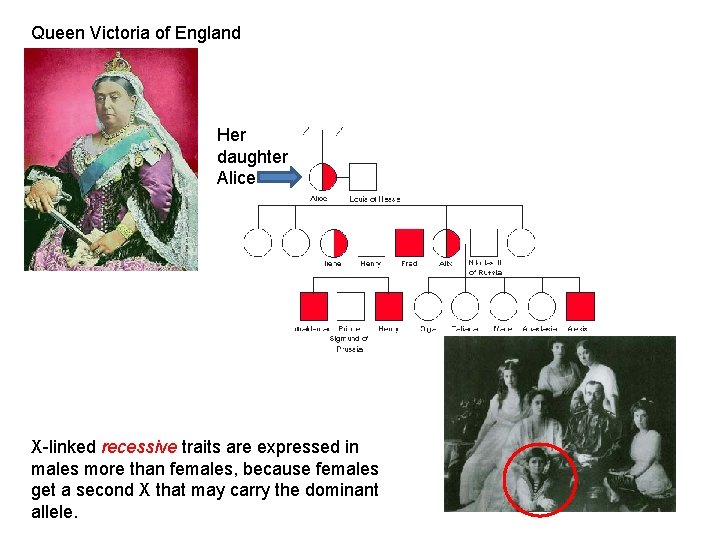
Queen Victoria of England Her daughter Alice X-linked recessive traits are expressed in males more than females, because females get a second X that may carry the dominant allele.

A. Sex Determination B. Sex Linkage C. Dosage Compensation - Females have two ‘doses’ of X-linked genes, while males have one ‘dose’. Since protein concentration is often important in protein function, how is this imbalance corrected?

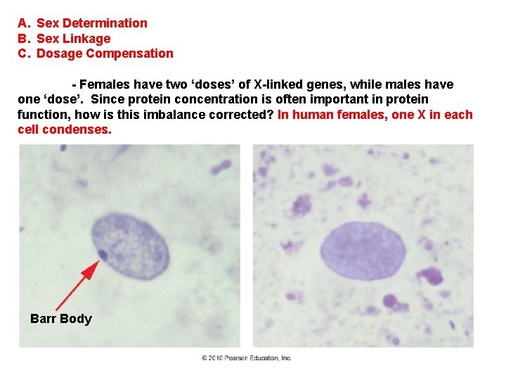
A. Sex Determination B. Sex Linkage C. Dosage Compensation - Females have two ‘doses’ of X-linked genes, while males have one ‘dose’. Since protein concentration is often important in protein function, how is this imbalance corrected? In human females, one X in each cell condenses. Barr Body

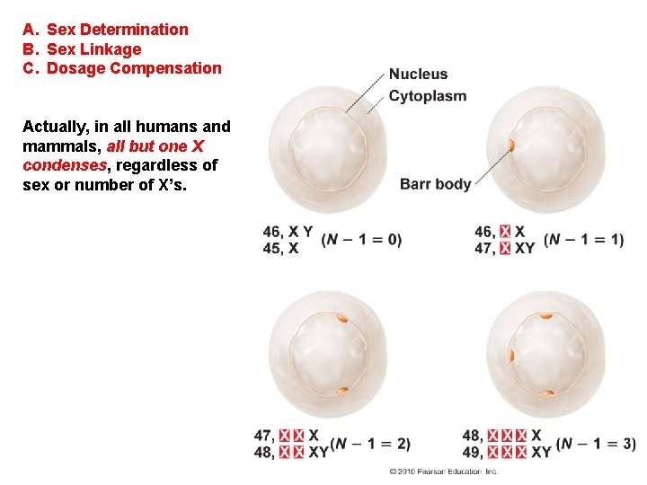
A. Sex Determination B. Sex Linkage C. Dosage Compensation Actually, in all humans and mammals, all but one X condenses, regardless of sex or number of X’s.

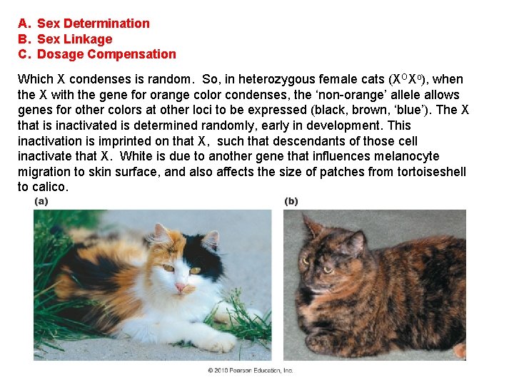
A. Sex Determination B. Sex Linkage C. Dosage Compensation Which X condenses is random. So, in heterozygous female cats (XOXo), when the X with the gene for orange color condenses, the ‘non-orange’ allele allows genes for other colors at other loci to be expressed (black, brown, ‘blue’). The X that is inactivated is determined randomly, early in development. This inactivation is imprinted on that X, such that descendants of those cell inactivate that X. White is due to another gene that influences melanocyte migration to skin surface, and also affects the size of patches from tortoiseshell to calico.

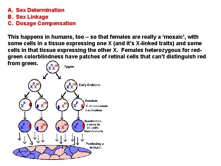
A. Sex Determination B. Sex Linkage C. Dosage Compensation This happens in humans, too – so that females are really a ‘mosaic’, with some cells in a tissue expressing one X (and it’s X-linked traits) and some cells in that tissue expressing the other X. Females heterozygous for redgreen colorblindness have patches of retinal cells that can’t distinguish red from green.

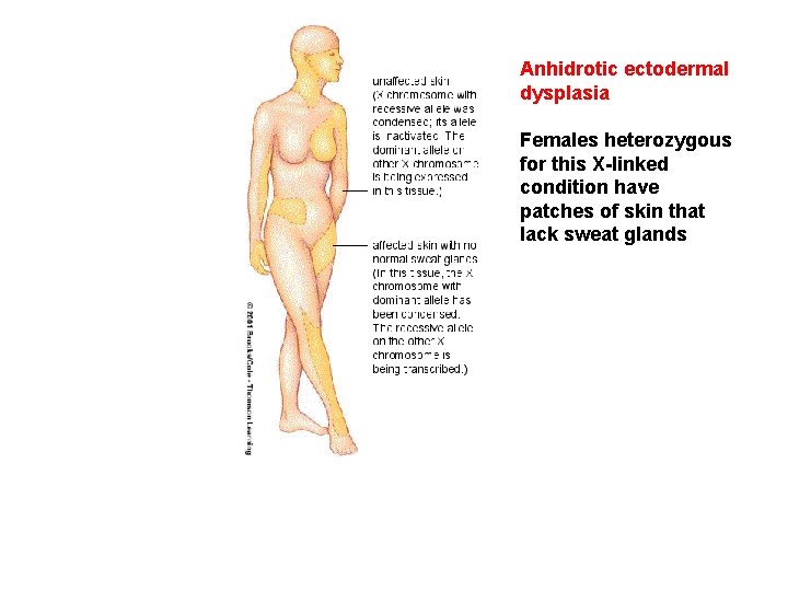
Anhidrotic ectodermal dysplasia Females heterozygous for this X-linked condition have patches of skin that lack sweat glands

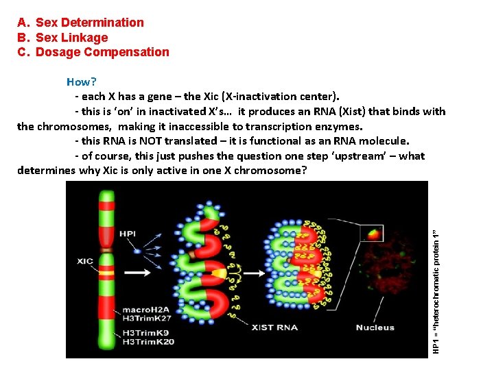
A. Sex Determination B. Sex Linkage C. Dosage Compensation HP 1 = “heterochromatic protein 1” How? - each X has a gene – the Xic (X-inactivation center). - this is ‘on’ in inactivated X’s… it produces an RNA (Xist) that binds with the chromosomes, making it inaccessible to transcription enzymes. - this RNA is NOT translated – it is functional as an RNA molecule. - of course, this just pushes the question one step ‘upstream’ – what determines why Xic is only active in one X chromosome?

A. Sex Determination B. Sex Linkage C. Dosage Compensation How? - each X has a gene – the Xic (X-inactivation center). - this is ‘on’ in inactivated X’s… it produces an RNA that binds with the X chromosomes, making it inaccessible to transcription enzymes. - this RNA is NOT translated – it is functional as an RNA molecule. - of course, this just pushes the question one step ‘upstream’ – what determines why Xic is only active in one X chromosome? When? - It seems to be an ‘imprinted’ phenomenon, so that daughter cells have the same X inactivated. However, this seems to happen at different points in development for different tissues.

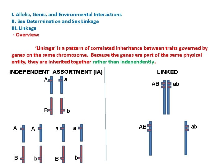
I. Allelic, Genic, and Environmental Interactions II. Sex Determination and Sex Linkage III. Linkage - Overview: ‘Linkage’ is a pattern of correlated inheritance between traits governed by genes on the same chromosome. Because the genes are part of the same physical entity, they are inherited together rather than independently. INDEPENDENT ASSORTMENT (IA) a A B A b LINKED AB ab b a B a b AB ab

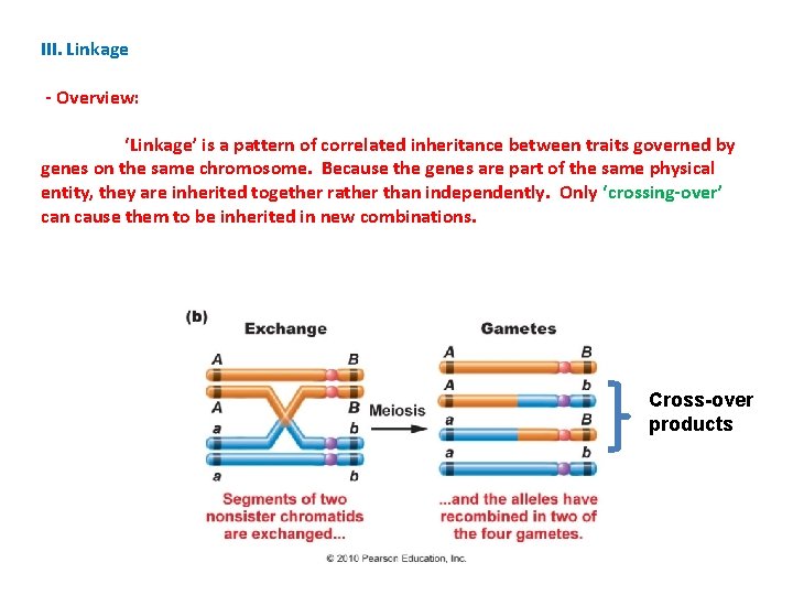
III. Linkage - Overview: ‘Linkage’ is a pattern of correlated inheritance between traits governed by genes on the same chromosome. Because the genes are part of the same physical entity, they are inherited together rather than independently. Only ‘crossing-over’ can cause them to be inherited in new combinations. Cross-over products

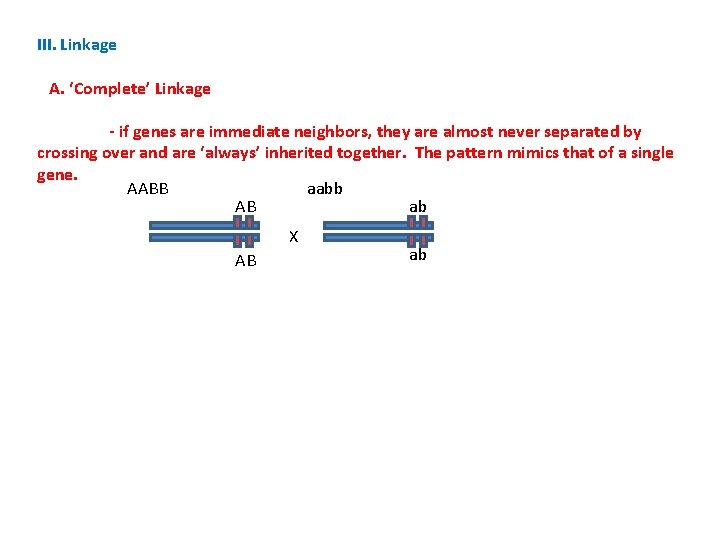
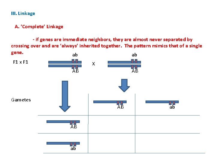
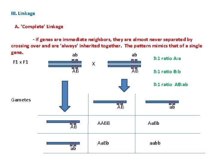
III. Linkage A. ‘Complete’ Linkage - if genes are immediate neighbors, they are almost never separated by crossing over and are ‘always’ inherited together. The pattern mimics that of a single gene. AABB aabb AB ab X AB ab

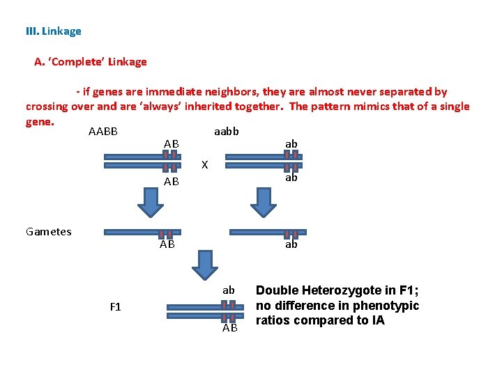
III. Linkage A. ‘Complete’ Linkage - if genes are immediate neighbors, they are almost never separated by crossing over and are ‘always’ inherited together. The pattern mimics that of a single gene. AABB aabb AB ab X ab AB Gametes AB ab ab F 1 AB Double Heterozygote in F 1; no difference in phenotypic ratios compared to IA

III. Linkage A. ‘Complete’ Linkage - if genes are immediate neighbors, they are almost never separated by crossing over and are ‘always’ inherited together. The pattern mimics that of a single gene. ab ab F 1 x F 1 X AB AB Gametes AB AB ab ab

III. Linkage A. ‘Complete’ Linkage - if genes are immediate neighbors, they are almost never separated by crossing over and are ‘always’ inherited together. The pattern mimics that of a single gene. ab ab 3: 1 ratio A: a F 1 x F 1 X AB AB 3: 1 ratio B: b 3: 1 ratio AB: ab Gametes AB AB ab ab AABB Aa. Bb aabb

III. Linkage A. ‘Complete’ Linkage B. ‘Incomplete’ Linkage

III. Linkage A. ‘Complete’ Linkage B. ‘Incomplete’ Linkage - Crossing over in a region is rare

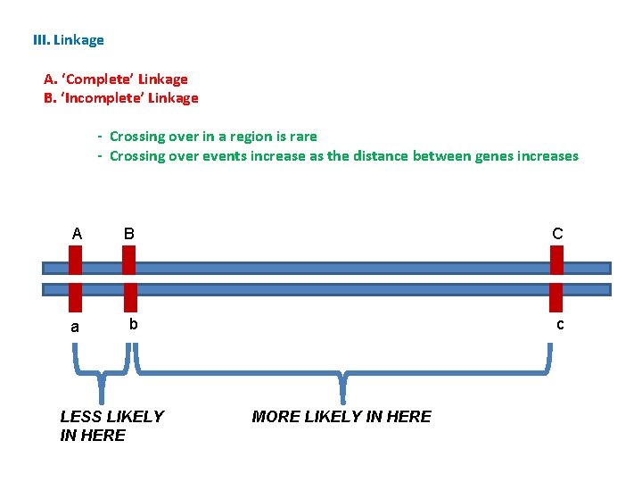
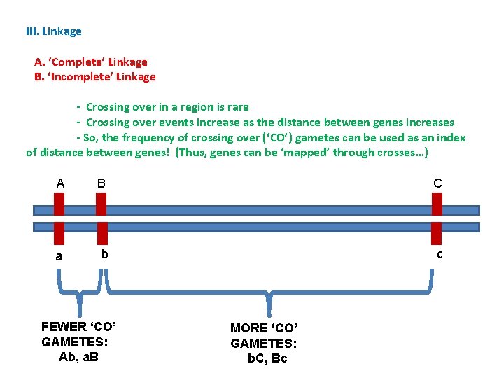
III. Linkage A. ‘Complete’ Linkage B. ‘Incomplete’ Linkage - Crossing over in a region is rare - Crossing over events increase as the distance between genes increases A B C a b c LESS LIKELY IN HERE MORE LIKELY IN HERE

III. Linkage A. ‘Complete’ Linkage B. ‘Incomplete’ Linkage - Crossing over in a region is rare - Crossing over events increase as the distance between genes increases - So, the frequency of crossing over (‘CO’) gametes can be used as an index of distance between genes! (Thus, genes can be ‘mapped’ through crosses…) A B C a b c FEWER ‘CO’ GAMETES: Ab, a. B MORE ‘CO’ GAMETES: b. C, Bc

III. Linkage A. ‘Complete’ Linkage B. ‘Incomplete’ Linkage - Crossing over in a region is rare - Crossing over events increase as the distance between genes increases - So, the frequency of crossing over (‘CO’) gametes can be used as an index of distance between genes! (Thus, genes can be ‘mapped’ through crosses…) - How can we measure the frequency of recombinant (‘cross-over’) gametes? Is there a type of cross where we can ‘see’ the frequency of different types of gametes produced by the heterozygote as they are expressed as the phenotypes of the offspring?

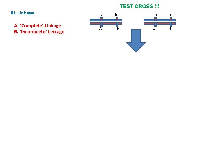
TEST CROSS !!! III. Linkage A. ‘Complete’ Linkage B. ‘Incomplete’ Linkage a A b B a a b b

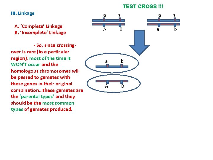
TEST CROSS !!! III. Linkage A. ‘Complete’ Linkage B. ‘Incomplete’ Linkage - So, since crossingover is rare (in a particular region), most of the time it WON’T occur and the homologous chromosomes will be passed to gametes with these genes in their original combination…these gametes are the ‘parental types’ and they should be the most common types of gametes produced. a A a b B a b A B a b b

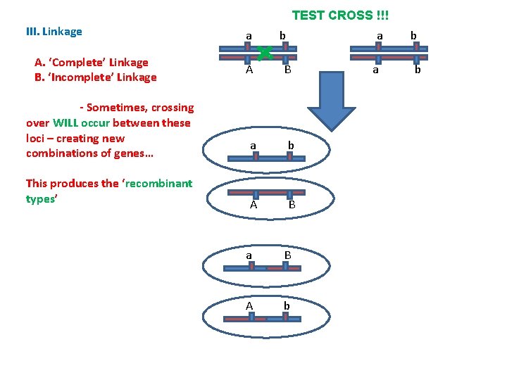
TEST CROSS !!! III. Linkage A. ‘Complete’ Linkage B. ‘Incomplete’ Linkage - Sometimes, crossing over WILL occur between these loci – creating new combinations of genes… This produces the ‘recombinant types’ a A a b B a b A B a B A b a b b

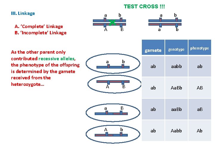
TEST CROSS !!! III. Linkage A. ‘Complete’ Linkage B. ‘Incomplete’ Linkage As the other parent only contributed recessive alleles, the phenotype of the offspring is determined by the gamete received from the heterozygote… a A a b a B a b A B b b gamete genotype phenotype ab aabb ab ab Aa. Bb AB a B ab aa. Bb a. B A b ab Aabb Ab

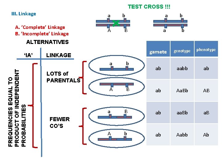
TEST CROSS !!! III. Linkage a A. ‘Complete’ Linkage B. ‘Incomplete’ Linkage A a b a B b b ALTERNATIVES FREQUENCIES EQUAL TO PRODUCT OF INDEPENDENT PROBABILITIES ‘IA’ LINKAGE a b A B LOTS of PARENTALS gamete genotype phenotype ab aabb ab ab Aa. Bb AB a B ab aa. Bb a. B A b ab Aabb Ab FEWER CO’S

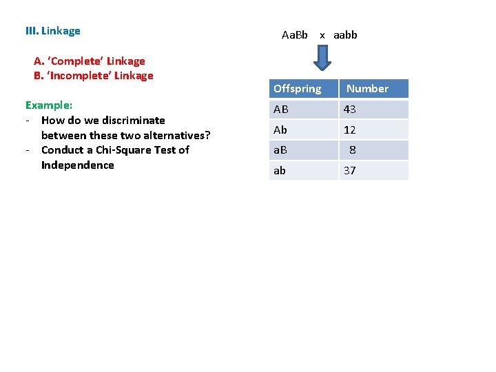
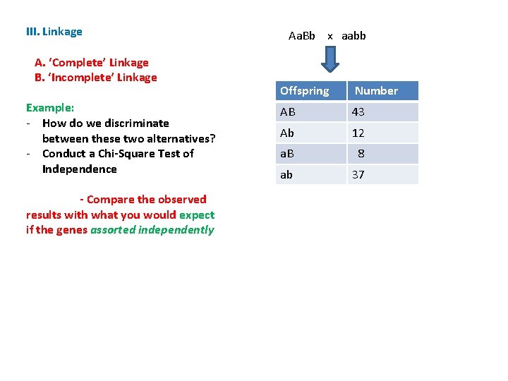
III. Linkage A. ‘Complete’ Linkage B. ‘Incomplete’ Linkage Example: - How do we discriminate between these two alternatives? - Conduct a Chi-Square Test of Independence Aa. Bb x aabb Offspring Number AB 43 Ab 12 a. B 8 ab 37

III. Linkage A. ‘Complete’ Linkage B. ‘Incomplete’ Linkage Example: - How do we discriminate between these two alternatives? - Conduct a Chi-Square Test of Independence - Compare the observed results with what you would expect if the genes assorted independently Aa. Bb x aabb Offspring Number AB 43 Ab 12 a. B 8 ab 37

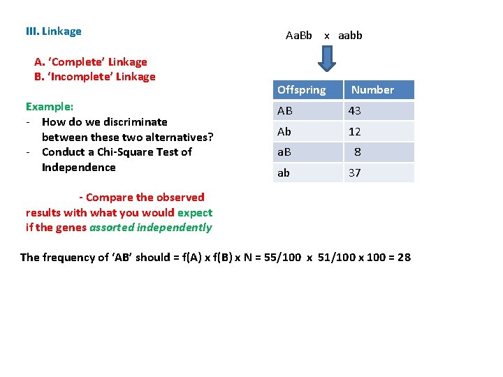
III. Linkage A. ‘Complete’ Linkage B. ‘Incomplete’ Linkage Example: - How do we discriminate between these two alternatives? - Conduct a Chi-Square Test of Independence Aa. Bb x aabb Offspring Number AB 43 Ab 12 a. B 8 ab 37 - Compare the observed results with what you would expect if the genes assorted independently The frequency of ‘AB’ should = f(A) x f(B) x N = 55/100 x 51/100 x 100 = 28

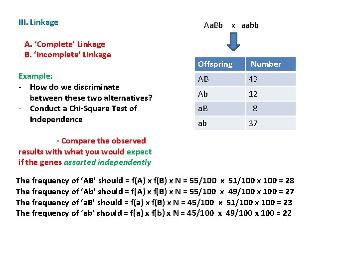
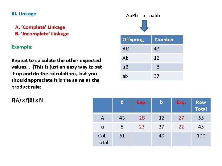
III. Linkage A. ‘Complete’ Linkage B. ‘Incomplete’ Linkage Example: - How do we discriminate between these two alternatives? - Conduct a Chi-Square Test of Independence Aa. Bb x aabb Offspring Number AB 43 Ab 12 a. B 8 ab 37 - Compare the observed results with what you would expect if the genes assorted independently The frequency of ‘AB’ should = f(A) x f(B) x N = 55/100 x 51/100 x 100 = 28 The frequency of ‘Ab’ should = f(A) x f(B) x N = 55/100 x 49/100 x 100 = 27 The frequency of ‘a. B’ should = f(a) x f(B) x N = 45/100 x 51/100 x 100 = 23 The frequency of ‘ab’ should = f(a) x f(b) x N = 45/100 x 49/100 x 100 = 22

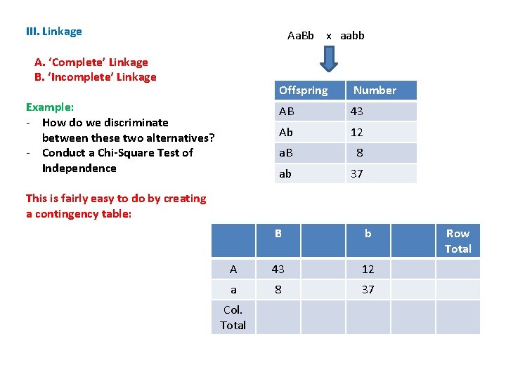
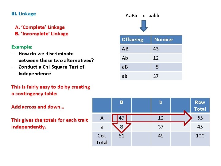
III. Linkage Aa. Bb x aabb A. ‘Complete’ Linkage B. ‘Incomplete’ Linkage Example: - How do we discriminate between these two alternatives? - Conduct a Chi-Square Test of Independence Offspring Number AB 43 Ab 12 a. B 8 ab 37 This is fairly easy to do by creating a contingency table: B b A 43 12 a 8 37 Col. Total Row Total

III. Linkage Aa. Bb x aabb A. ‘Complete’ Linkage B. ‘Incomplete’ Linkage Example: - How do we discriminate between these two alternatives? - Conduct a Chi-Square Test of Independence Offspring Number AB 43 Ab 12 a. B 8 ab 37 This is fairly easy to do by creating a contingency table: B b Row Total A 43 12 55 a 8 37 45 Col. Total 51 49 100 Add across and down… This gives the totals for each trait independently.

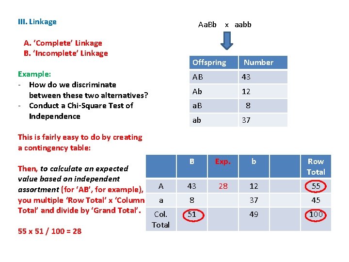
III. Linkage Aa. Bb x aabb A. ‘Complete’ Linkage B. ‘Incomplete’ Linkage Example: - How do we discriminate between these two alternatives? - Conduct a Chi-Square Test of Independence Offspring Number AB 43 Ab 12 a. B 8 ab 37 This is fairly easy to do by creating a contingency table: Then, to calculate an expected value based on independent assortment (for ‘AB’, for example), you multiple ‘Row Total’ x ‘Column Total’ and divide by ‘Grand Total’. 55 x 51 / 100 = 28 B Exp. b Row Total A 43 28 12 55 a 8 37 45 Col. Total 51 49 100

III. Linkage Aa. Bb x aabb A. ‘Complete’ Linkage B. ‘Incomplete’ Linkage Offspring Number Example: AB 43 Repeat to calculate the other expected values… (This is just an easy way to set it up and do the calculations, but you should appreciate it is the same as the product rule: Ab 12 a. B 8 ab 37 F(A) x f(B) x N B Exp. b Exp. Row Total A 43 28 12 27 55 a 8 23 37 22 45 Col. Total 51 49 100

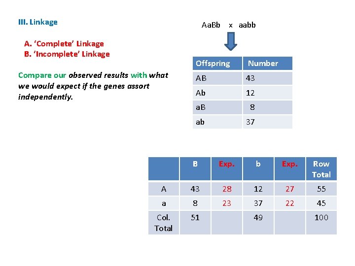
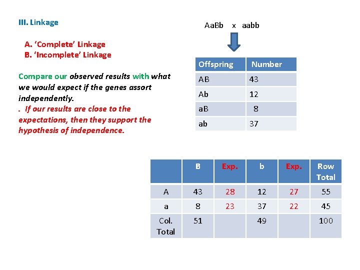
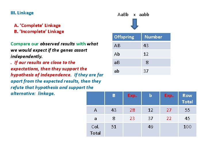
III. Linkage Aa. Bb x aabb A. ‘Complete’ Linkage B. ‘Incomplete’ Linkage Compare our observed results with what we would expect if the genes assort independently. Offspring Number AB 43 Ab 12 a. B 8 ab 37 B Exp. b Exp. Row Total A 43 28 12 27 55 a 8 23 37 22 45 Col. Total 51 49 100

III. Linkage Aa. Bb x aabb A. ‘Complete’ Linkage B. ‘Incomplete’ Linkage Compare our observed results with what we would expect if the genes assort independently. . If our results are close to the expectations, then they support the hypothesis of independence. Offspring Number AB 43 Ab 12 a. B 8 ab 37 B Exp. b Exp. Row Total A 43 28 12 27 55 a 8 23 37 22 45 Col. Total 51 49 100

III. Linkage Aa. Bb x aabb A. ‘Complete’ Linkage B. ‘Incomplete’ Linkage Compare our observed results with what we would expect if the genes assort independently. . If our results are close to the expectations, then they support the hypothesis of independence. If they are far apart from the expected results, then they refute that hypothesis and support the alternative: linkage. Offspring Number AB 43 Ab 12 a. B 8 ab 37 B Exp. b Exp. Row Total A 43 28 12 27 55 a 8 23 37 22 45 Col. Total 51 49 100

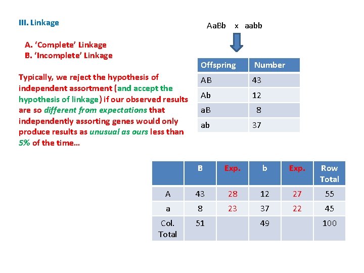
III. Linkage Aa. Bb x aabb A. ‘Complete’ Linkage B. ‘Incomplete’ Linkage Typically, we reject the hypothesis of independent assortment (and accept the hypothesis of linkage) if our observed results are so different from expectations that independently assorting genes would only produce results as unusual as ours less than 5% of the time… Offspring Number AB 43 Ab 12 a. B 8 ab 37 B Exp. b Exp. Row Total A 43 28 12 27 55 a 8 23 37 22 45 Col. Total 51 49 100

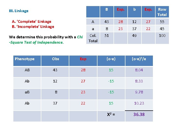
B Exp. b Exp. Row Total A 43 28 12 27 55 a 8 23 37 22 45 Col. Total 51 III. Linkage A. ‘Complete’ Linkage B. ‘Incomplete’ Linkage We determine this probability with a Chi -Square Test of Independence. Phenotype 49 Obs Exp (o-e)2/e AB 43 28 15 8. 04 Ab 12 27 -15 8. 33 a. B 8 23 -15 9. 78 Ab 37 22 15 10. 23 X 2 = 36. 38 100

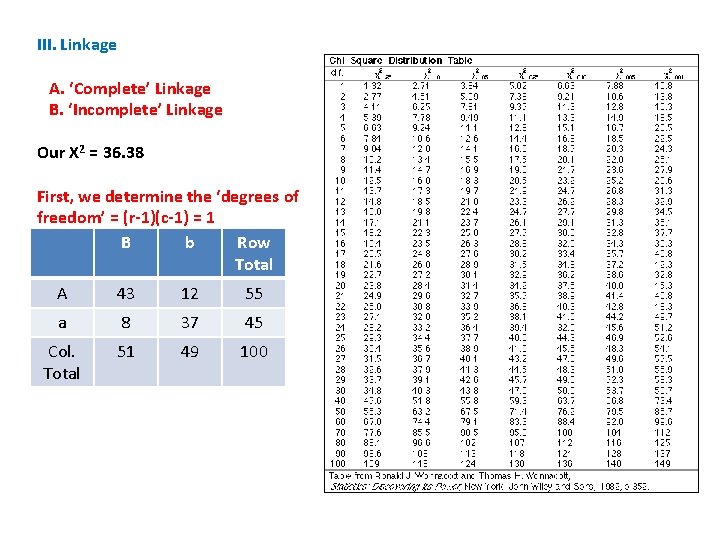
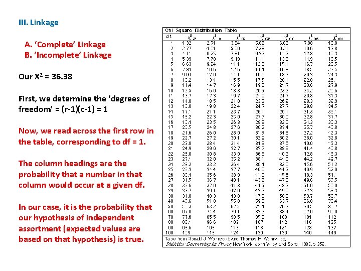
III. Linkage A. ‘Complete’ Linkage B. ‘Incomplete’ Linkage Our X 2 = 36. 38 First, we determine the ‘degrees of freedom’ = (r-1)(c-1) = 1 B b Row Total A 43 12 55 a 8 37 45 Col. Total 51 49 100

III. Linkage A. ‘Complete’ Linkage B. ‘Incomplete’ Linkage Our X 2 = 36. 38 First, we determine the ‘degrees of freedom’ = (r-1)(c-1) = 1 Now, we read across the first row in the table, corresponding to df = 1. The column headings are the probability that a number in that column would occur at a given df. In our case, it is the probability that our hypothesis of independent assortment (expected values are based on that hypothesis) is true.

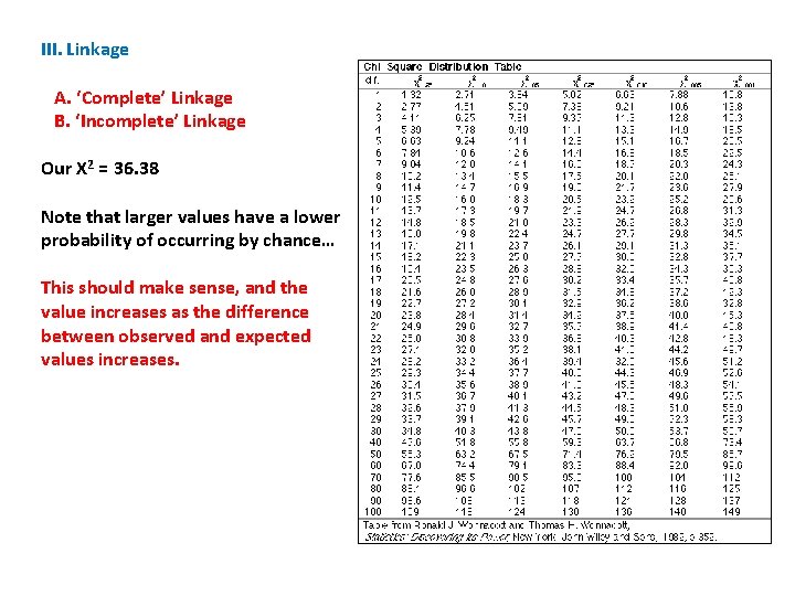
III. Linkage A. ‘Complete’ Linkage B. ‘Incomplete’ Linkage Our X 2 = 36. 38 Note that larger values have a lower probability of occurring by chance… This should make sense, and the value increases as the difference between observed and expected values increases.

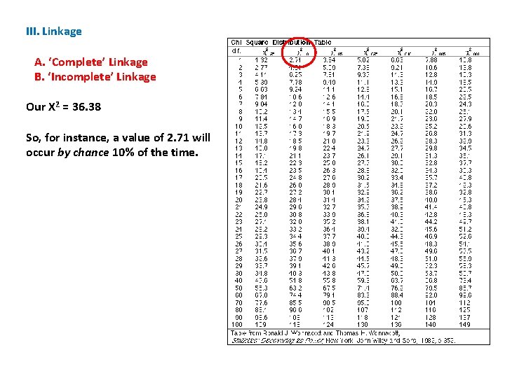
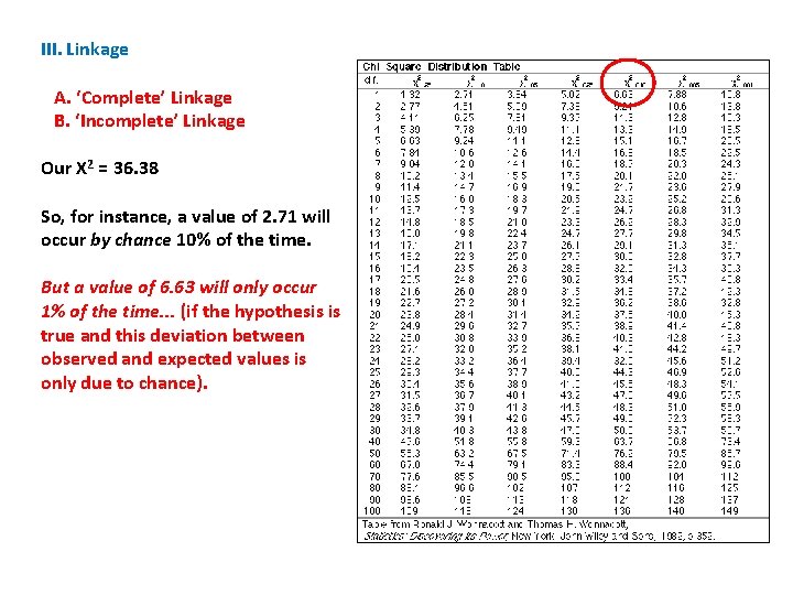
III. Linkage A. ‘Complete’ Linkage B. ‘Incomplete’ Linkage Our X 2 = 36. 38 So, for instance, a value of 2. 71 will occur by chance 10% of the time.

III. Linkage A. ‘Complete’ Linkage B. ‘Incomplete’ Linkage Our X 2 = 36. 38 So, for instance, a value of 2. 71 will occur by chance 10% of the time. But a value of 6. 63 will only occur 1% of the time. . . (if the hypothesis is true and this deviation between observed and expected values is only due to chance).

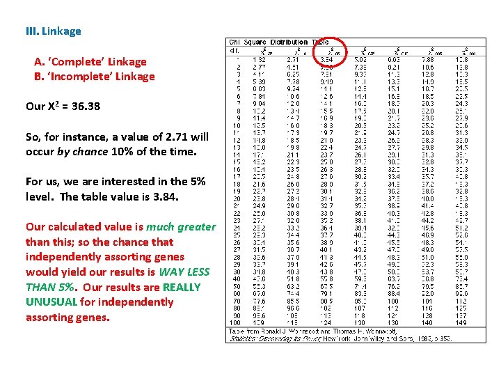
III. Linkage A. ‘Complete’ Linkage B. ‘Incomplete’ Linkage Our X 2 = 36. 38 So, for instance, a value of 2. 71 will occur by chance 10% of the time. For us, we are interested in the 5% level. The table value is 3. 84. Our calculated value is much greater than this; so the chance that independently assorting genes would yield our results is WAY LESS THAN 5%. Our results are REALLY UNUSUAL for independently assorting genes.

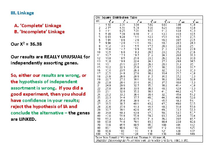
III. Linkage A. ‘Complete’ Linkage B. ‘Incomplete’ Linkage Our X 2 = 36. 38 Our results are REALLY UNUSUAL for independently assorting genes. So, either our results are wrong, or the hypothesis of independent assortment is wrong. If you did a good experiment, then you should have confidence in your results; reject the hypothesis of IA and conclude the alternative – the genes are LINKED.

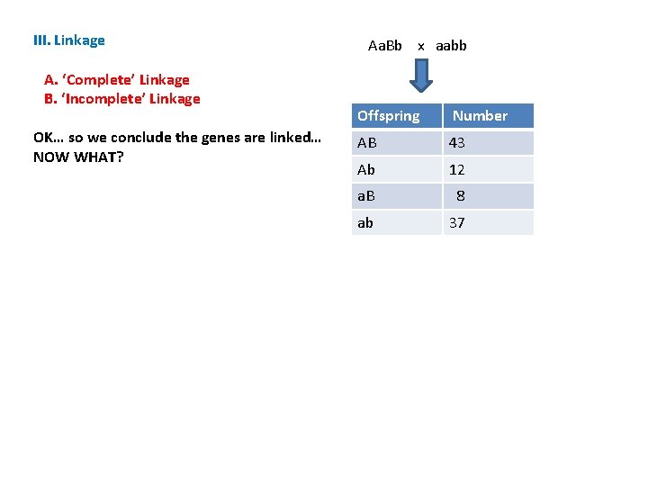
III. Linkage A. ‘Complete’ Linkage B. ‘Incomplete’ Linkage OK… so we conclude the genes are linked… NOW WHAT? Aa. Bb x aabb Offspring Number AB 43 Ab 12 a. B 8 ab 37