A general agnostic active learning algorithm Claire Monteleoni

A general agnostic active learning algorithm Claire Monteleoni UC San Diego Joint work with Sanjoy Dasgupta and Daniel Hsu, UCSD.

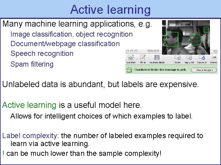
Active learning Many machine learning applications, e. g. Image classification, object recognition Document/webpage classification Speech recognition Spam filtering Unlabeled data is abundant, but labels are expensive. Active learning is a useful model here. Allows for intelligent choices of which examples to label. Label complexity: the number of labeled examples required to learn via active learning. ! can be much lower than the sample complexity!

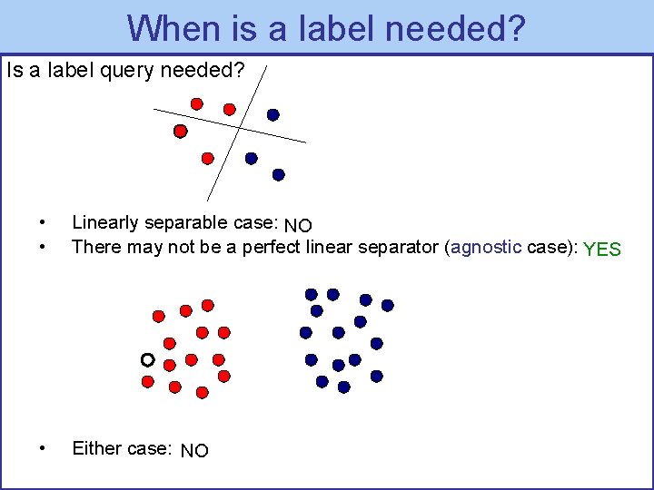
When is a label needed? Is a label query needed? • • Linearly separable case: NO There may not be a perfect linear separator (agnostic case): YES • Either case: NO

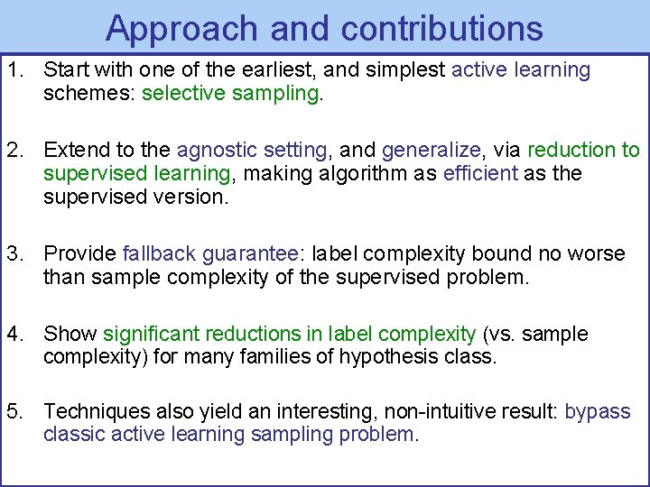
Approach and contributions 1. Start with one of the earliest, and simplest active learning schemes: selective sampling. 2. Extend to the agnostic setting, and generalize, via reduction to supervised learning, making algorithm as efficient as the supervised version. 3. Provide fallback guarantee: label complexity bound no worse than sample complexity of the supervised problem. 4. Show significant reductions in label complexity (vs. sample complexity) for many families of hypothesis class. 5. Techniques also yield an interesting, non-intuitive result: bypass classic active learning sampling problem.

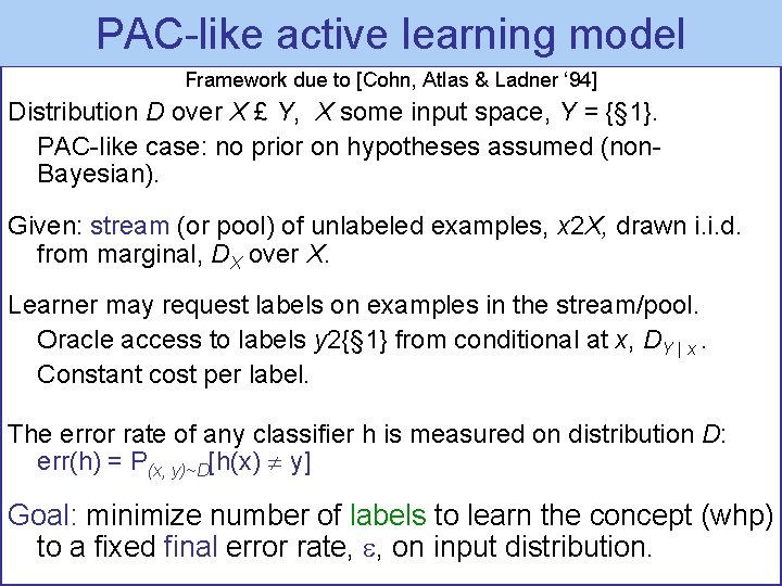
PAC-like selective activesampling learning framework model Framework due to [Cohn, Atlas & Ladner ‘ 94] Distribution D over X £ Y, X some input space, Y = {§ 1}. PAC-like case: no prior on hypotheses assumed (non. Bayesian). Given: stream (or pool) of unlabeled examples, x 2 X, drawn i. i. d. from marginal, DX over X. Learner may request labels on examples in the stream/pool. Oracle access to labels y 2{§ 1} from conditional at x, DY | x. Constant cost per label. The error rate of any classifier h is measured on distribution D: err(h) = P(x, y)~D[h(x) y] Goal: minimize number of labels to learn the concept (whp) to a fixed final error rate, , on input distribution.

Selective sampling algorithm Region of uncertainty [CAL ‘ 94]: subset of data space for which there exist hypotheses (in H) consistent with all previous data, that disagree. Example: hypothesis class, H = {linear separators}. Separable assumption. Algorithm: Selective sampling [Cohn, Atlas & Ladner ‘ 94] (orig. NIPS 1989): For each point in the stream, if point falls in region of uncertainty, request label. Easy to represent the region of uncertainty for certain, separable problems. BUT, in this work we address: - What about agnostic case? ! Reduction! - General hypothesis classes?

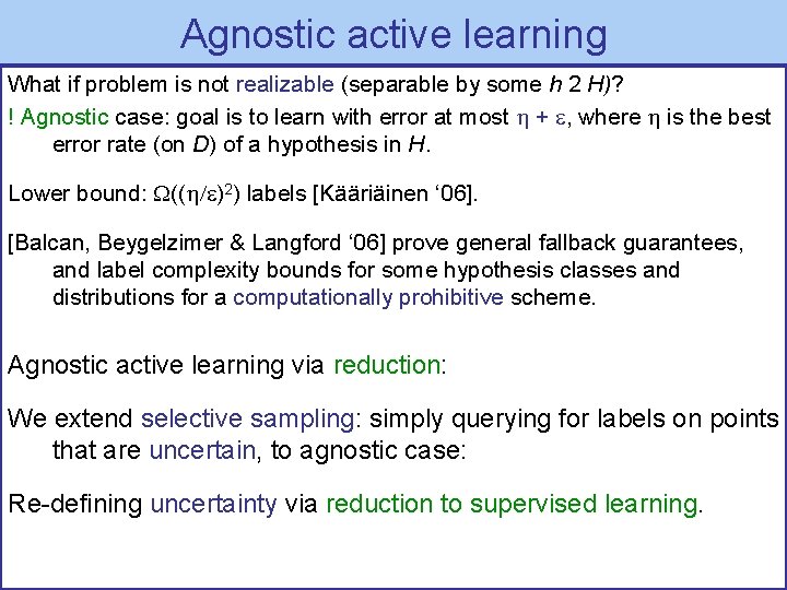
Agnostic active learning What if problem is not realizable (separable by some h 2 H)? ! Agnostic case: goal is to learn with error at most + , where is the best error rate (on D) of a hypothesis in H. Lower bound: (( )2) labels [Kääriäinen ‘ 06]. [Balcan, Beygelzimer & Langford ‘ 06] prove general fallback guarantees, and label complexity bounds for some hypothesis classes and distributions for a computationally prohibitive scheme. Agnostic active learning via reduction: We extend selective sampling: simply querying for labels on points that are uncertain, to agnostic case: Re-defining uncertainty via reduction to supervised learning.

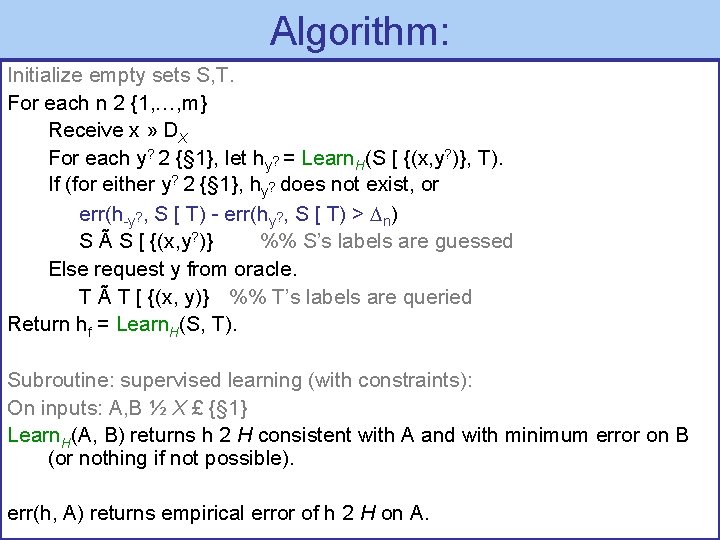
Algorithm: Initialize empty sets S, T. For each n 2 {1, …, m} Receive x » DX For each y? 2 {§ 1}, let hy? = Learn. H(S [ {(x, y? )}, T). If (for either y? 2 {§ 1}, hy? does not exist, or err(h-y? , S [ T) - err(hy? , S [ T) > n) S Ã S [ {(x, y? )} %% S’s labels are guessed Else request y from oracle. T Ã T [ {(x, y)} %% T’s labels are queried Return hf = Learn. H(S, T). Subroutine: supervised learning (with constraints): On inputs: A, B ½ X £ {§ 1} Learn. H(A, B) returns h 2 H consistent with A and with minimum error on B (or nothing if not possible). err(h, A) returns empirical error of h 2 H on A.

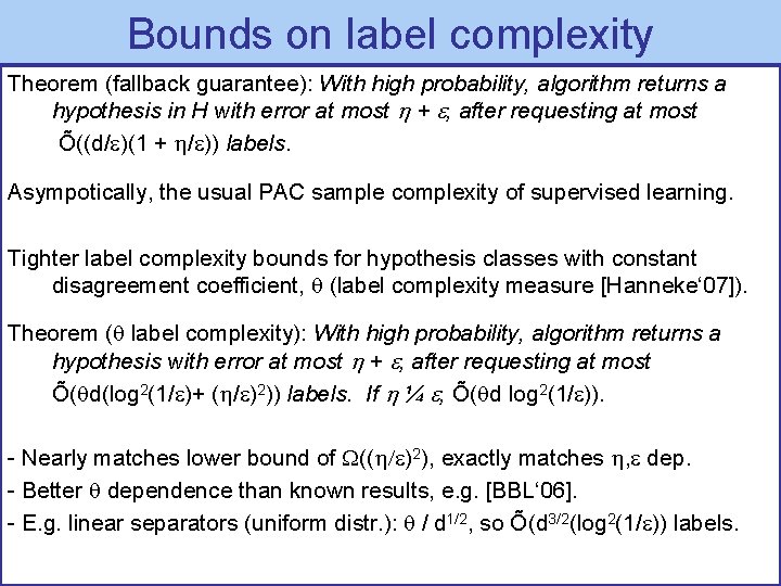
Bounds on label complexity Theorem (fallback guarantee): With high probability, algorithm returns a hypothesis in H with error at most + , after requesting at most Õ((d/ )(1 + / )) labels. Asympotically, the usual PAC sample complexity of supervised learning. Tighter label complexity bounds for hypothesis classes with constant disagreement coefficient, (label complexity measure [Hanneke‘ 07]). Theorem ( label complexity): With high probability, algorithm returns a hypothesis with error at most + , after requesting at most Õ( d(log 2(1/ )+ ( / )2)) labels. If ¼ , Õ( d log 2(1/ )). - Nearly matches lower bound of (( )2), exactly matches , dep. - Better dependence than known results, e. g. [BBL‘ 06]. - E. g. linear separators (uniform distr. ): / d 1/2, so Õ(d 3/2(log 2(1/ )) labels.

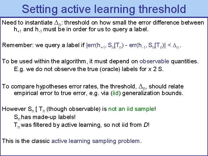
Setting active learning threshold Need to instantiate n: threshold on how small the error difference between h+1 and h-1 must be in order for us to query a label. Remember: we query a label if |err(h+1, Sn[Tn) - err(h-1, Sn[Tn)| < n. To be used within the algorithm, it must depend on observable quantities. E. g. we do not observe the true (oracle) labels for x 2 S. To compare hypotheses error rates, the threshold, n, should relate empirical error to true error, e. g. via (iid) generalization bounds. However Sn [ Tn (though observable) is not an iid sample! Sn has made-up labels! Tn was filtered by active learning, so not iid from D! This is the classic active learning sampling problem.

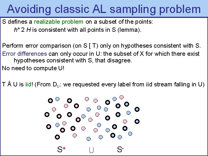
Avoiding classic AL sampling problem S defines a realizable problem on a subset of the points: h* 2 H is consistent with all points in S (lemma). Perform error comparison (on S [ T) only on hypotheses consistent with S. Error differences can only occur in U: the subset of X for which there exist hypotheses consistent with S, that disagree. No need to compute U! T Å U is iid! (From DU: we requested every label from iid stream falling in U) S+ U S-

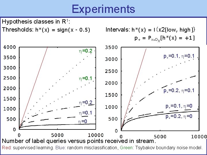
Experiments Hypothesis classes in R 1: Thresholds: h*(x) = sign(x - 0. 5) Intervals: h*(x) = I(x 2[low, high]) p+ = Px» DX[h*(x) = +1] =0. 2 p+=0. 1, =0. 1 p+=0. 2, =0. 1 =0. 2 =0. 1 =0 p+=0. 1, =0 p+=0. 2, =0 Number of label queries versus points received in stream. Red: supervised learning. Blue: random misclassification, Green: Tsybakov boundary noise model.

Experiments Interval in R 1: h*(x) = I(x 2[0. 4, 0. 6]) Interval in R 2 (Axis-parallel boxes): h*(x) = I(x 2[0. 15, 0. 85]2) Label queries: 1 -400: 0 0 0. 5 1 All label queries (1 -2141). 0 0. 2 0. 4 0. 6 0. 8 Temporal breakdown of label request locations. Queries: 1 -200, 201 -400, 401 -509. 1

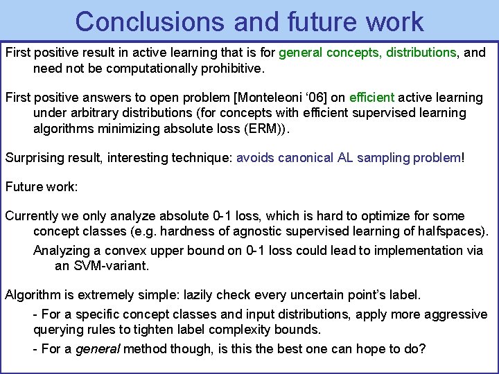
Conclusions and future work First positive result in active learning that is for general concepts, distributions, and need not be computationally prohibitive. First positive answers to open problem [Monteleoni ‘ 06] on efficient active learning under arbitrary distributions (for concepts with efficient supervised learning algorithms minimizing absolute loss (ERM)). Surprising result, interesting technique: avoids canonical AL sampling problem! Future work: Currently we only analyze absolute 0 -1 loss, which is hard to optimize for some concept classes (e. g. hardness of agnostic supervised learning of halfspaces). Analyzing a convex upper bound on 0 -1 loss could lead to implementation via an SVM-variant. Algorithm is extremely simple: lazily check every uncertain point’s label. - For a specific concept classes and input distributions, apply more aggressive querying rules to tighten label complexity bounds. - For a general method though, is the best one can hope to do?

Thank you! And thanks to coauthors: Sanjoy Dasgupta Daniel Hsu

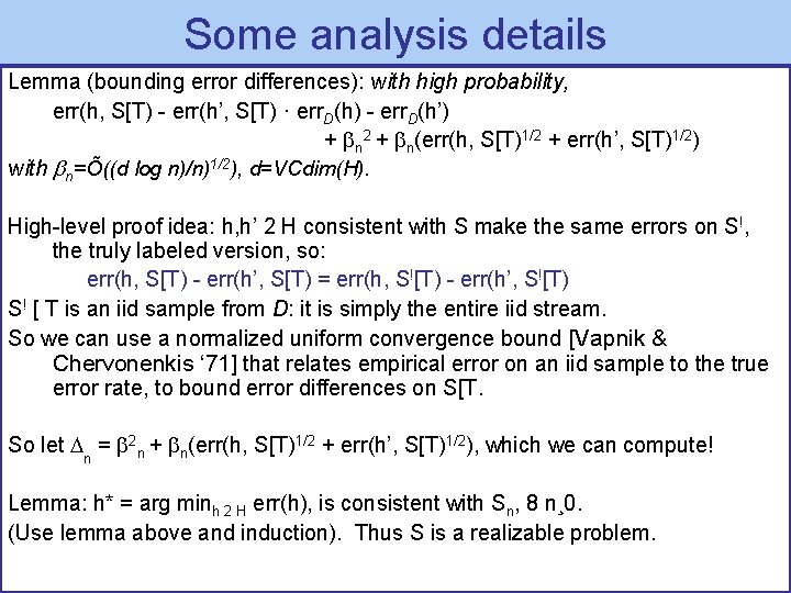
Some analysis details Lemma (bounding error differences): with high probability, err(h, S[T) - err(h’, S[T) · err. D(h) - err. D(h’) + n 2 + n(err(h, S[T)1/2 + err(h’, S[T)1/2) with n=Õ((d log n)/n)1/2), d=VCdim(H). High-level proof idea: h, h’ 2 H consistent with S make the same errors on S!, the truly labeled version, so: err(h, S[T) - err(h’, S[T) = err(h, S![T) - err(h’, S![T) S! [ T is an iid sample from D: it is simply the entire iid stream. So we can use a normalized uniform convergence bound [Vapnik & Chervonenkis ‘ 71] that relates empirical error on an iid sample to the true error rate, to bound error differences on S[T. So let n = 2 n + n(err(h, S[T)1/2 + err(h’, S[T)1/2), which we can compute! Lemma: h* = arg minh 2 H err(h), is consistent with Sn, 8 n¸ 0. (Use lemma above and induction). Thus S is a realizable problem.