5 Stereo Reconstruction Slides from A Zisserman S
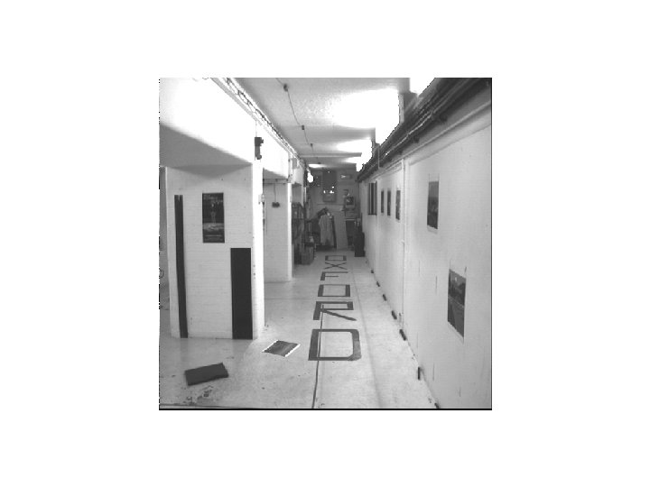
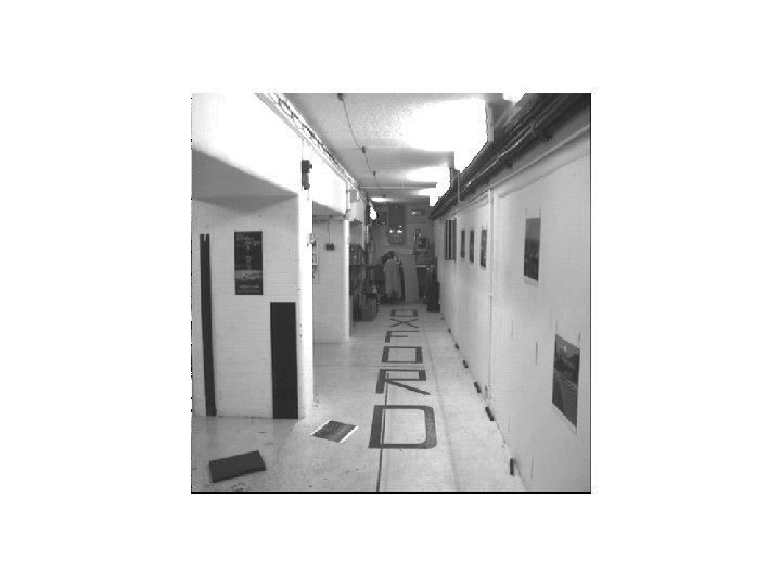

- Slides: 118

5 – Stereo Reconstruction Slides from A. Zisserman & S. Lazebnik

Overview • Single camera geometry • Recap of Homogenous coordinates • Perspective projection model • Camera calibration • Stereo Reconstruction • Epipolar geometry • Stereo correspondence • Triangulation

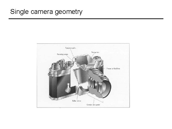
Single camera geometry

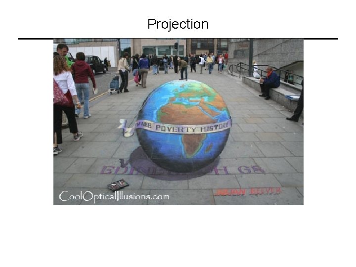
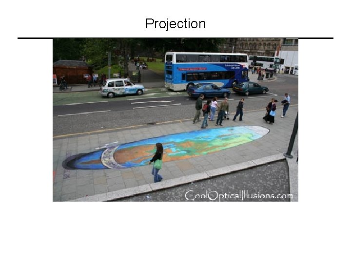
Projection

Projection

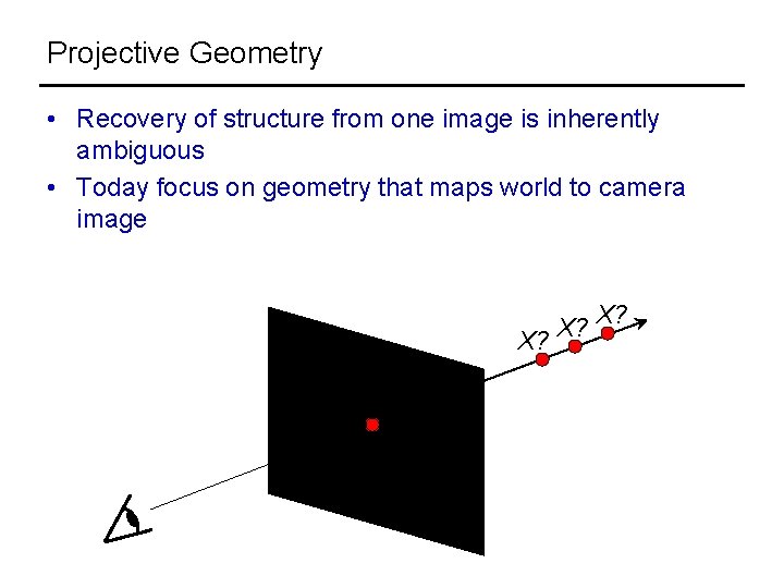
Projective Geometry • Recovery of structure from one image is inherently ambiguous • Today focus on geometry that maps world to camera image X? X? X? x

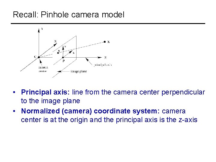
Recall: Pinhole camera model • Principal axis: line from the camera center perpendicular to the image plane • Normalized (camera) coordinate system: camera center is at the origin and the principal axis is the z-axis

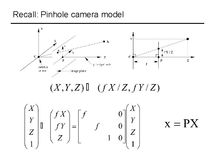
Recall: Pinhole camera model

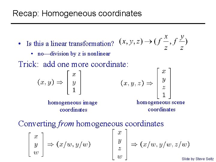
Recap: Homogeneous coordinates • Is this a linear transformation? • no—division by z is nonlinear Trick: add one more coordinate: homogeneous image coordinates homogeneous scene coordinates Converting from homogeneous coordinates Slide by Steve Seitz

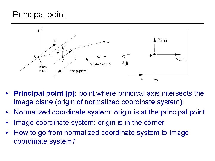
Principal point • Principal point (p): point where principal axis intersects the image plane (origin of normalized coordinate system) • Normalized coordinate system: origin is at the principal point • Image coordinate system: origin is in the corner • How to go from normalized coordinate system to image coordinate system?

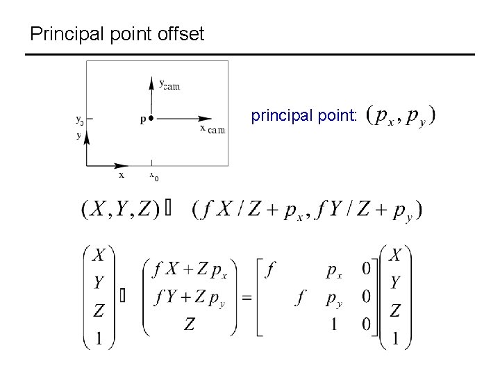
Principal point offset principal point:

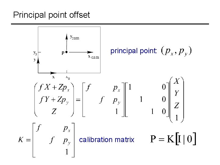
Principal point offset principal point: calibration matrix

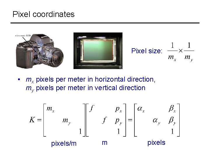
Pixel coordinates Pixel size: • mx pixels per meter in horizontal direction, my pixels per meter in vertical direction pixels/m m pixels

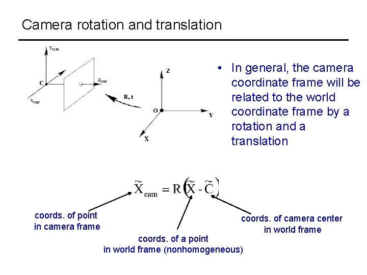
Camera rotation and translation • In general, the camera coordinate frame will be related to the world coordinate frame by a rotation and a translation coords. of point in camera frame coords. of camera center in world frame coords. of a point in world frame (nonhomogeneous)

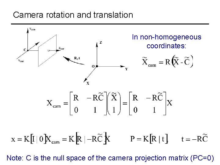
Camera rotation and translation In non-homogeneous coordinates: Note: C is the null space of the camera projection matrix (PC=0)

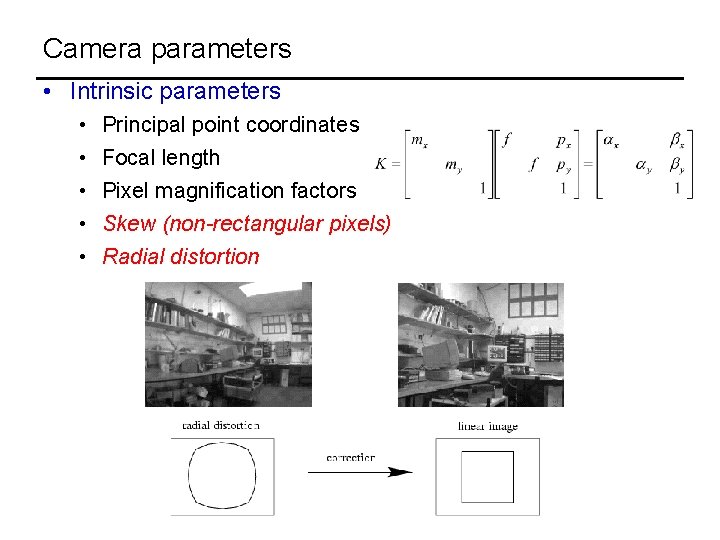
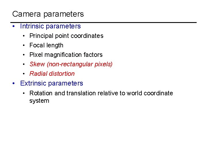
Camera parameters • Intrinsic parameters • • • Principal point coordinates Focal length Pixel magnification factors Skew (non-rectangular pixels) Radial distortion

Camera parameters • Intrinsic parameters • • • Principal point coordinates Focal length Pixel magnification factors Skew (non-rectangular pixels) Radial distortion • Extrinsic parameters • Rotation and translation relative to world coordinate system

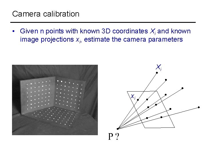
Camera calibration • Given n points with known 3 D coordinates Xi and known image projections xi, estimate the camera parameters Xi xi

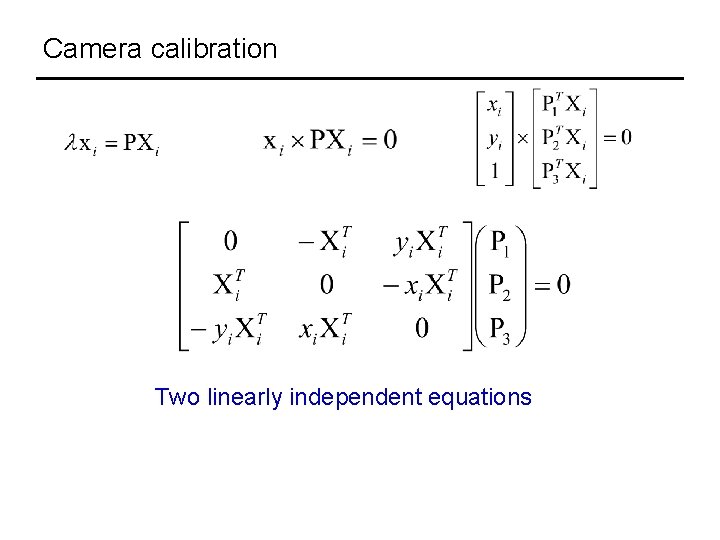
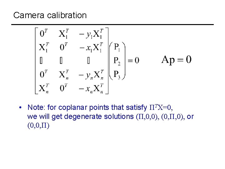
Camera calibration Two linearly independent equations

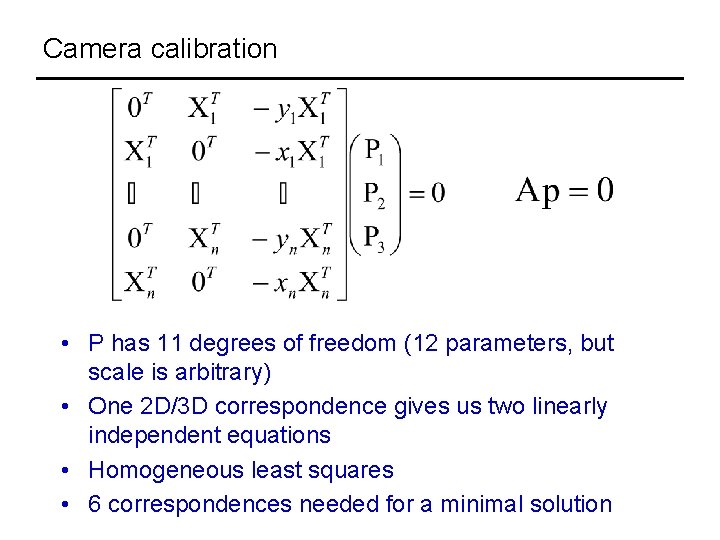
Camera calibration • P has 11 degrees of freedom (12 parameters, but scale is arbitrary) • One 2 D/3 D correspondence gives us two linearly independent equations • Homogeneous least squares • 6 correspondences needed for a minimal solution

Camera calibration • Note: for coplanar points that satisfy ΠTX=0, we will get degenerate solutions (Π, 0, 0), (0, Π, 0), or (0, 0, Π)

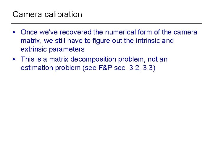
Camera calibration • Once we’ve recovered the numerical form of the camera matrix, we still have to figure out the intrinsic and extrinsic parameters • This is a matrix decomposition problem, not an estimation problem (see F&P sec. 3. 2, 3. 3)

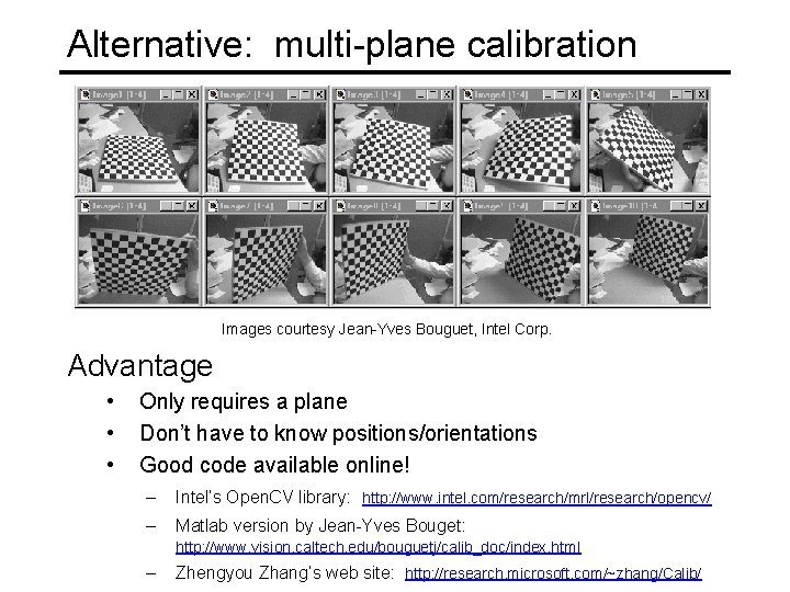
Alternative: multi-plane calibration Images courtesy Jean-Yves Bouguet, Intel Corp. Advantage • • • Only requires a plane Don’t have to know positions/orientations Good code available online! – Intel’s Open. CV library: http: //www. intel. com/research/mrl/research/opencv/ – Matlab version by Jean-Yves Bouget: http: //www. vision. caltech. edu/bouguetj/calib_doc/index. html CSE 576, Spring 2008 Projective Geometry 23 – Zhengyou Zhang’s web site: http: //research. microsoft. com/~zhang/Calib/

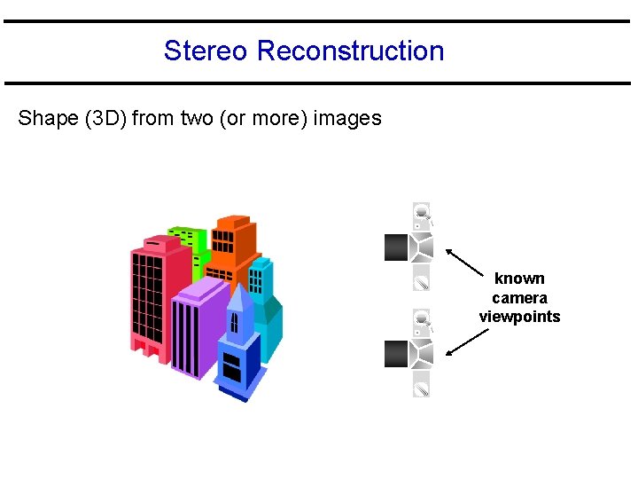
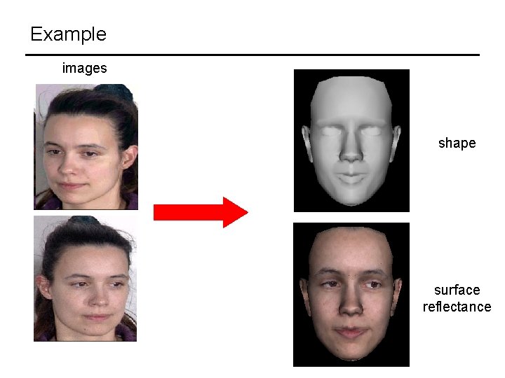
Stereo Reconstruction Shape (3 D) from two (or more) images known camera viewpoints

Example images shape surface reflectance

Scenarios The two images can arise from • A stereo rig consisting of two cameras • the two images are acquired simultaneously or • A single moving camera (static scene) • the two images are acquired sequentially The two scenarios are geometrically equivalent

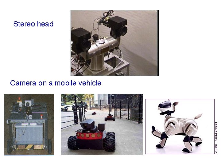
Stereo head Camera on a mobile vehicle

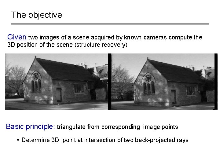
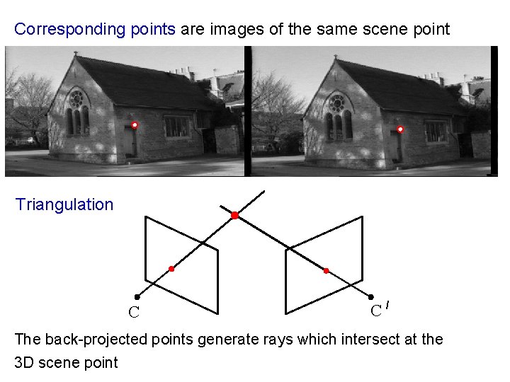
The objective Given two images of a scene acquired by known cameras compute the 3 D position of the scene (structure recovery) Basic principle: triangulate from corresponding image points • Determine 3 D point at intersection of two back-projected rays

Corresponding points are images of the same scene point Triangulation C C/ The back-projected points generate rays which intersect at the 3 D scene point

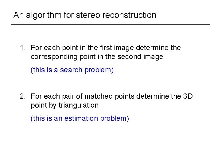
An algorithm for stereo reconstruction 1. For each point in the first image determine the corresponding point in the second image (this is a search problem) 2. For each pair of matched points determine the 3 D point by triangulation (this is an estimation problem)

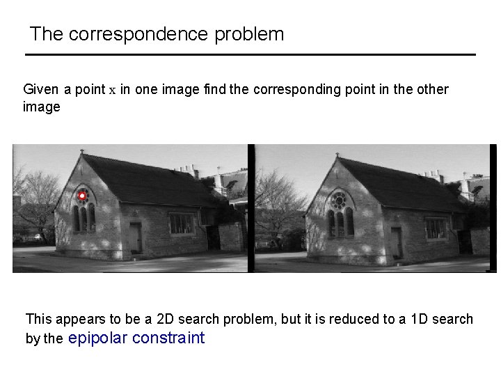
The correspondence problem Given a point x in one image find the corresponding point in the other image This appears to be a 2 D search problem, but it is reduced to a 1 D search by the epipolar constraint

Outline 1. Epipolar geometry • • the geometry of two cameras reduces the correspondence problem to a line search 2. Stereo correspondence algorithms 3. Triangulation

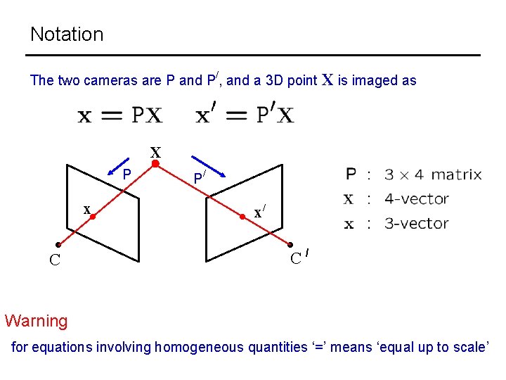
Notation / The two cameras are P and P , and a 3 D point X is imaged as X P x C P/ x/ C/ Warning for equations involving homogeneous quantities ‘=’ means ‘equal up to scale’

Epipolar geometry

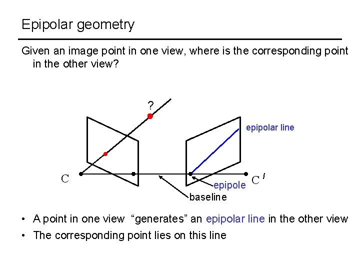
Epipolar geometry Given an image point in one view, where is the corresponding point in the other view? ? epipolar line C / C epipole baseline • A point in one view “generates” an epipolar line in the other view • The corresponding point lies on this line

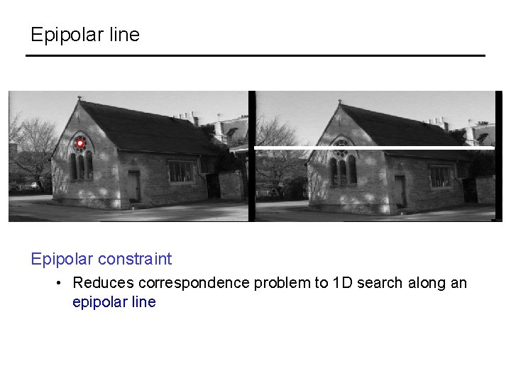
Epipolar line Epipolar constraint • Reduces correspondence problem to 1 D search along an epipolar line

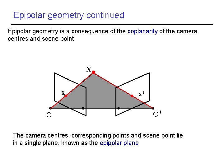
Epipolar geometry continued Epipolar geometry is a consequence of the coplanarity of the camera centres and scene point X x C x/ C/ The camera centres, corresponding points and scene point lie in a single plane, known as the epipolar plane

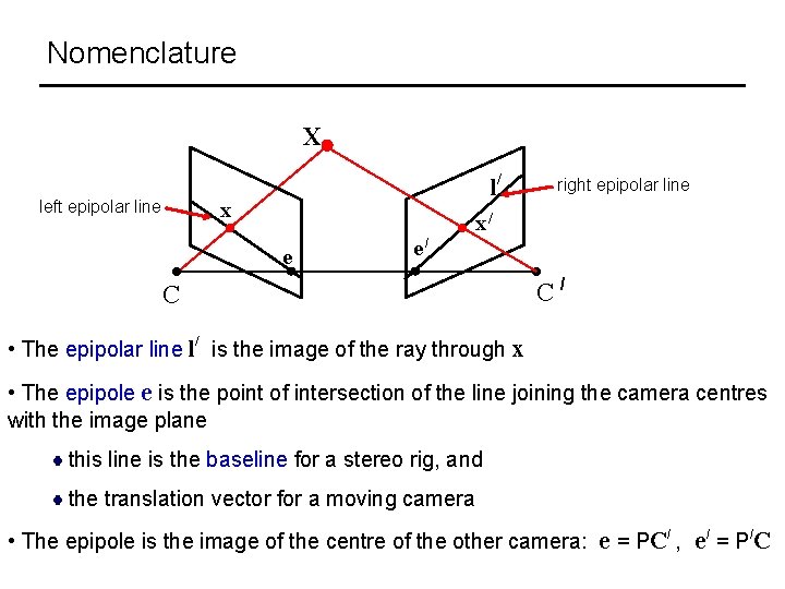
Nomenclature X left epipolar line l/ x right epipolar line x/ e e/ C C/ • The epipolar line l/ is the image of the ray through x • The epipole e is the point of intersection of the line joining the camera centres with the image plane this line is the baseline for a stereo rig, and the translation vector for a moving camera • The epipole is the image of the centre of the other camera: e = PC/ , e/ = P/C

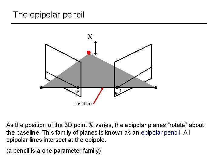
The epipolar pencil X e e / baseline As the position of the 3 D point X varies, the epipolar planes “rotate” about the baseline. This family of planes is known as an epipolar pencil. All epipolar lines intersect at the epipole. (a pencil is a one parameter family)

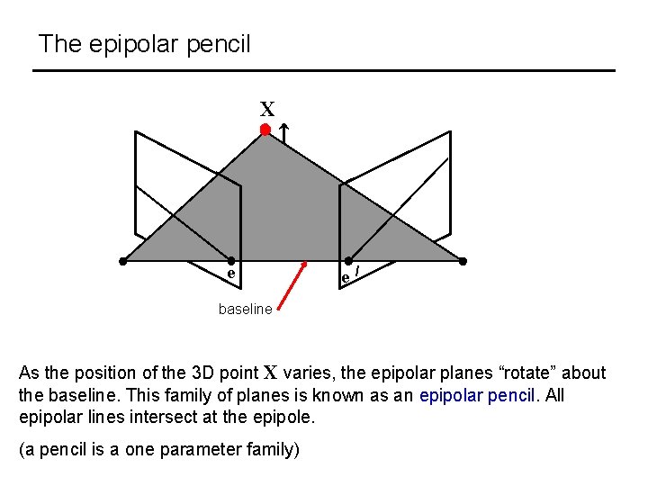
The epipolar pencil X e e / baseline As the position of the 3 D point X varies, the epipolar planes “rotate” about the baseline. This family of planes is known as an epipolar pencil. All epipolar lines intersect at the epipole. (a pencil is a one parameter family)

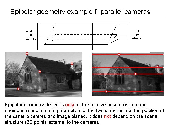
Epipolar geometry example I: parallel cameras Epipolar geometry depends only on the relative pose (position and orientation) and internal parameters of the two cameras, i. e. the position of the camera centres and image planes. It does not depend on the scene structure (3 D points external to the camera).

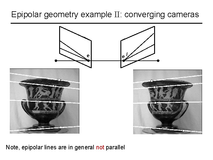
Epipolar geometry example II: converging cameras e e Note, epipolar lines are in general not parallel /

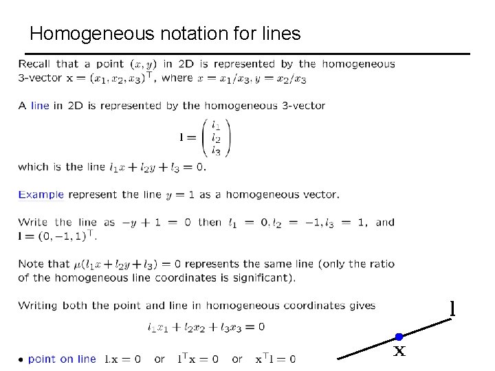
Homogeneous notation for lines

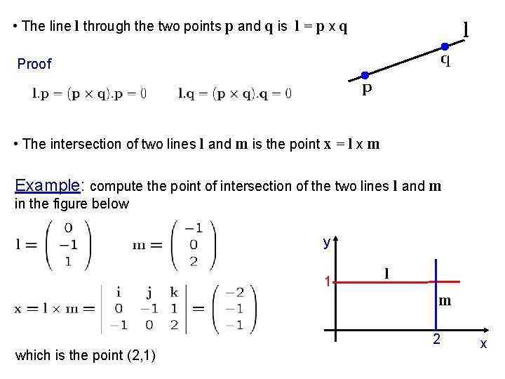
• The line l through the two points p and q is l = p x q Proof • The intersection of two lines l and m is the point x = l x m Example: compute the point of intersection of the two lines l and m in the figure below y 1 l m 2 which is the point (2, 1) x

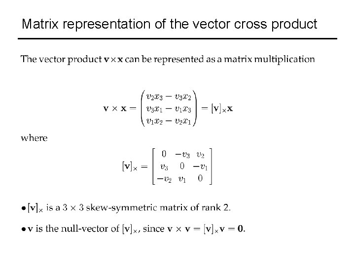
Matrix representation of the vector cross product

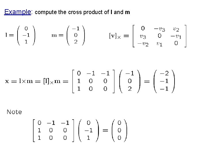
Example: compute the cross product of l and m

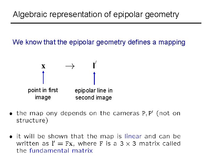
Algebraic representation of epipolar geometry We know that the epipolar geometry defines a mapping / x l point in first image epipolar line in second image

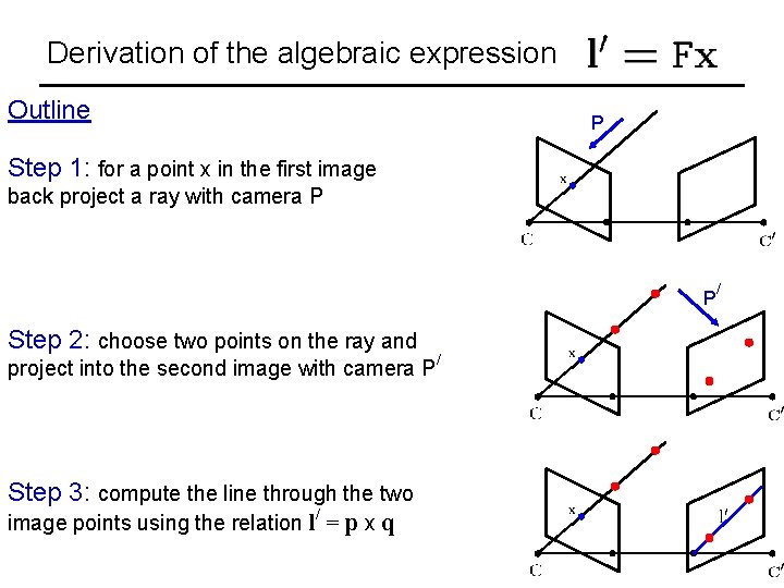
Derivation of the algebraic expression Outline P Step 1: for a point x in the first image back project a ray with camera P P Step 2: choose two points on the ray and project into the second image with camera P/ Step 3: compute the line through the two image points using the relation l/ = p x q /

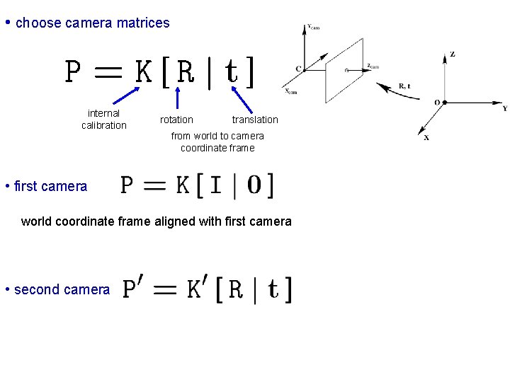
• choose camera matrices internal calibration rotation translation from world to camera coordinate frame • first camera world coordinate frame aligned with first camera • second camera

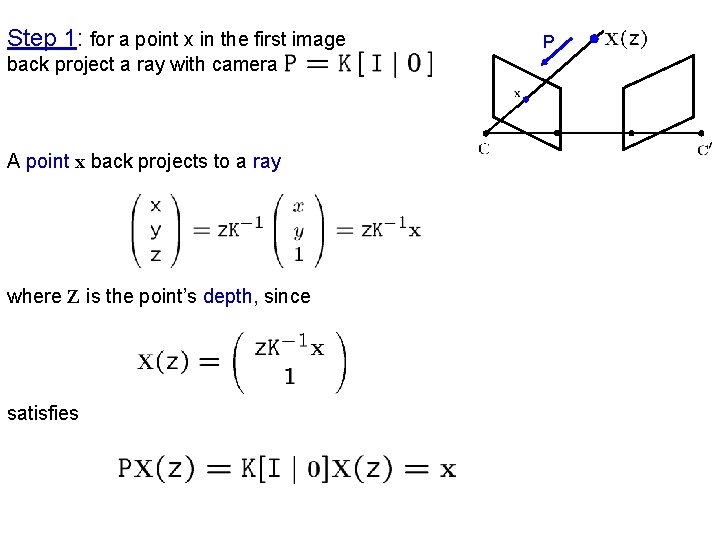
Step 1: for a point x in the first image back project a ray with camera A point x back projects to a ray where Z is the point’s depth, since satisfies P

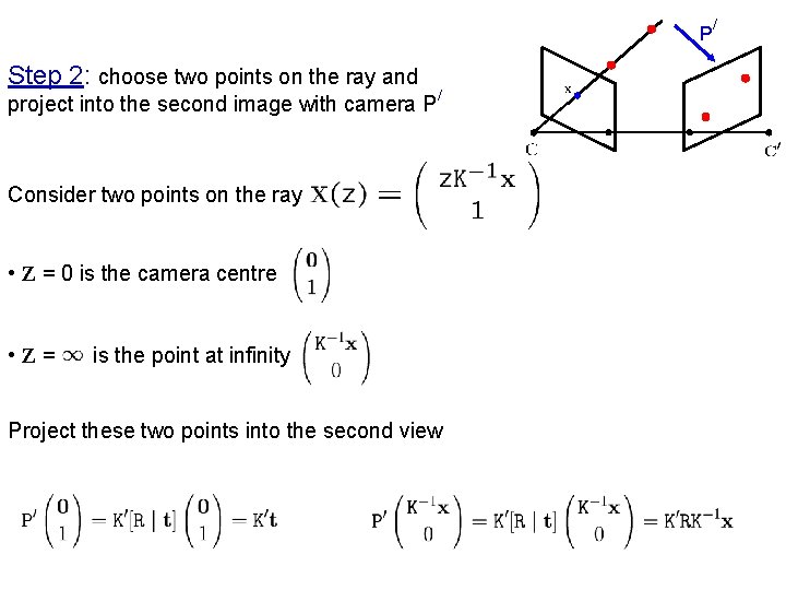
P Step 2: choose two points on the ray and project into the second image with camera P/ Consider two points on the ray • Z = 0 is the camera centre • Z= is the point at infinity Project these two points into the second view /

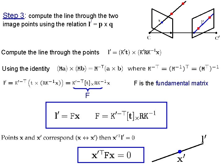
Step 3: compute the line through the two image points using the relation l/ = p x q Compute the line through the points Using the identity F is the fundamental matrix F

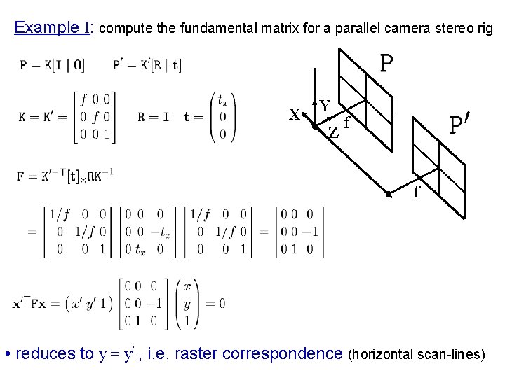
Example I: compute the fundamental matrix for a parallel camera stereo rig X Y Z f f • reduces to y = y/ , i. e. raster correspondence (horizontal scan-lines)

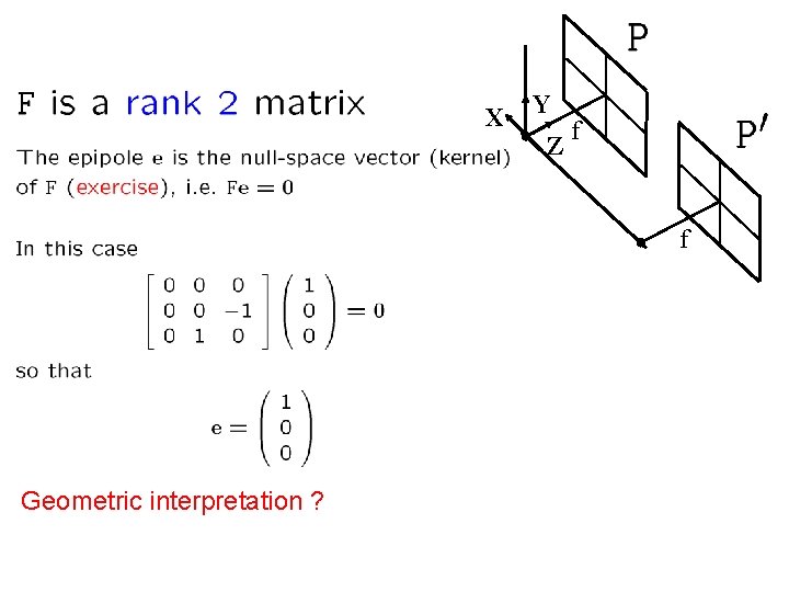
X Y Z f f Geometric interpretation ?

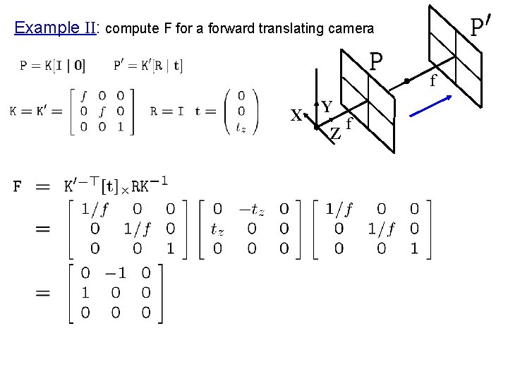
Example II: compute F for a forward translating camera f X Y Z f

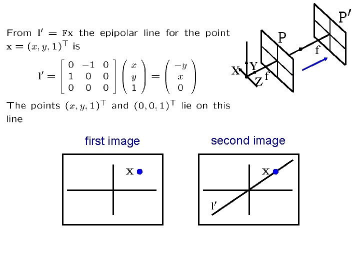
f X Y f Z first image second image


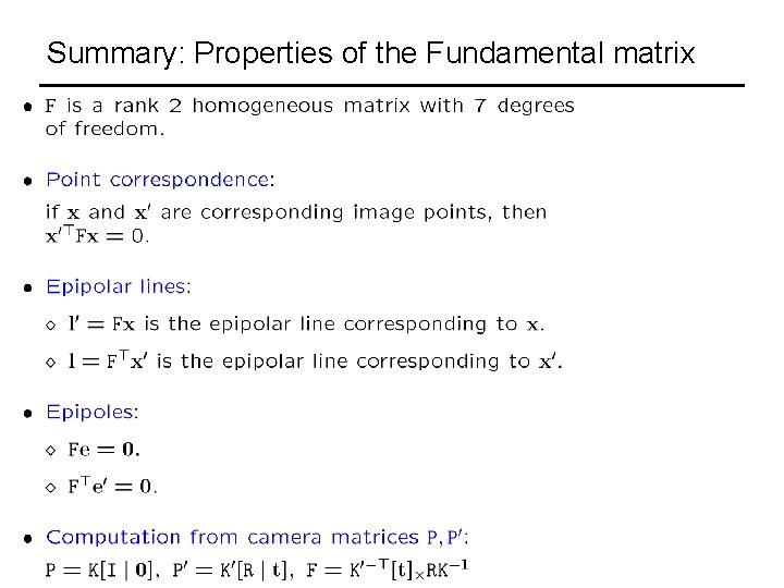
Summary: Properties of the Fundamental matrix

Admin Interlude • Assignment 1 due next week at start of class • Office hours right after class! • Meet Hao Li (haoli@cs. nyu. edu) whos is the class TA • Who did not get my class emails? • Please come and (legibly!) give me your email again.

Stereo correspondence algorithms

Problem statement Given: two images and their associated cameras compute corresponding image points. Algorithms may be classified into two types: 1. Dense: compute a correspondence at every pixel 2. Sparse: compute correspondences only for features The methods may be top down or bottom up

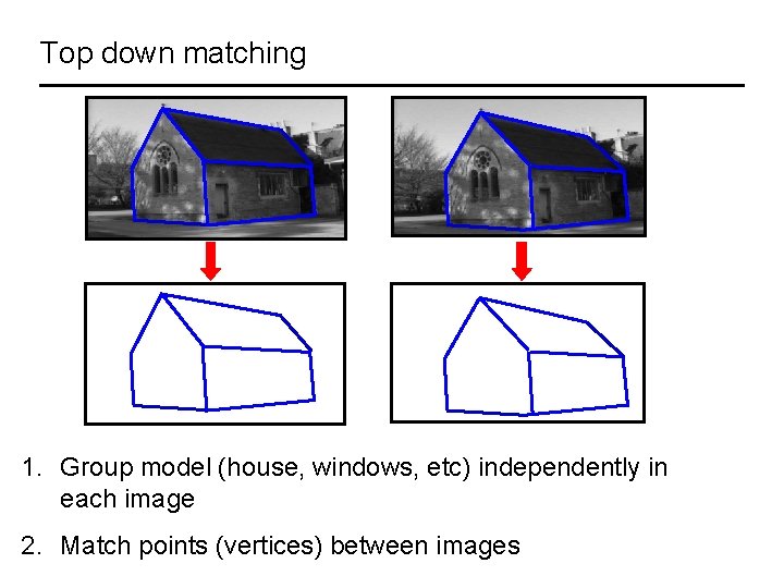
Top down matching 1. Group model (house, windows, etc) independently in each image 2. Match points (vertices) between images

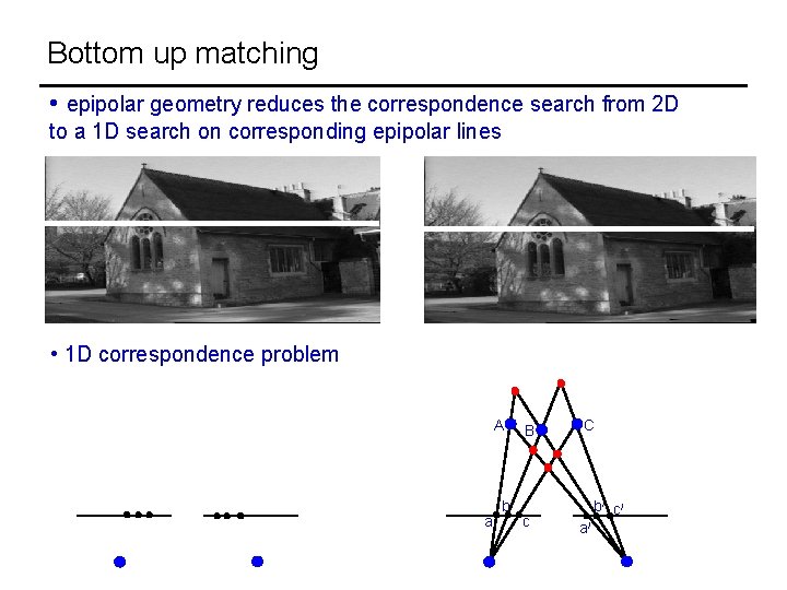
Bottom up matching • epipolar geometry reduces the correspondence search from 2 D to a 1 D search on corresponding epipolar lines • 1 D correspondence problem A a b B c C b/ c/ a/


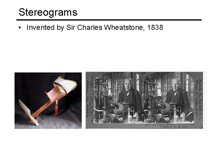
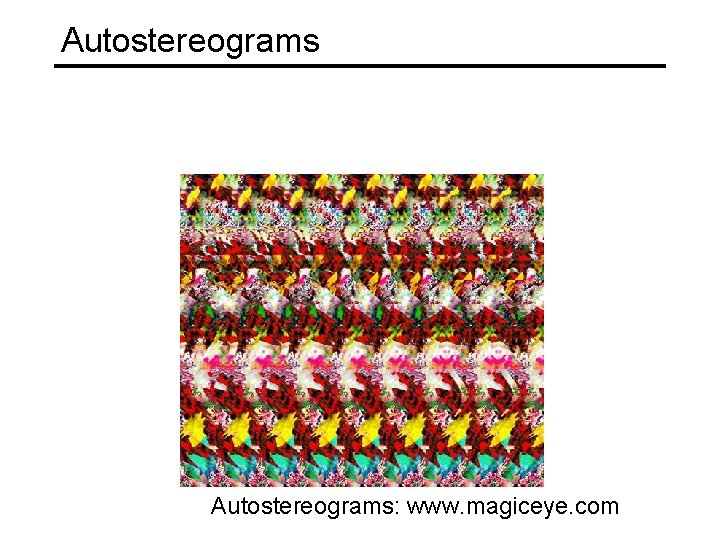
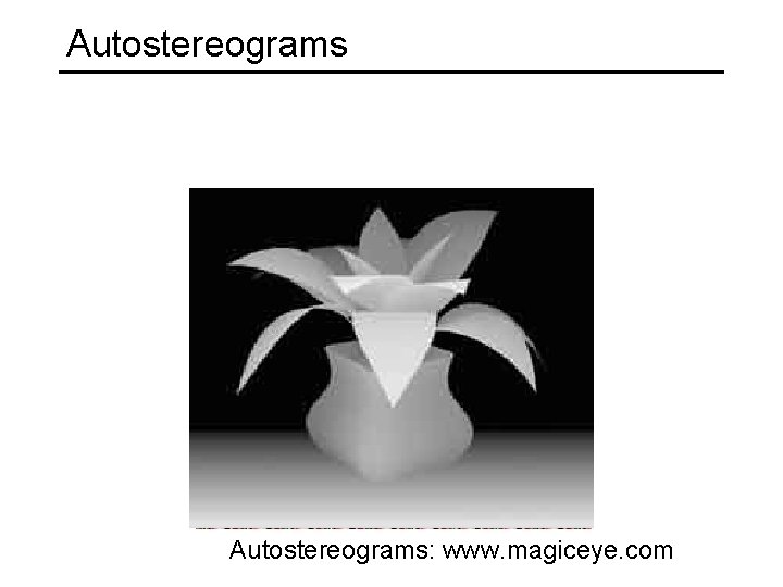
Stereograms • Invented by Sir Charles Wheatstone, 1838

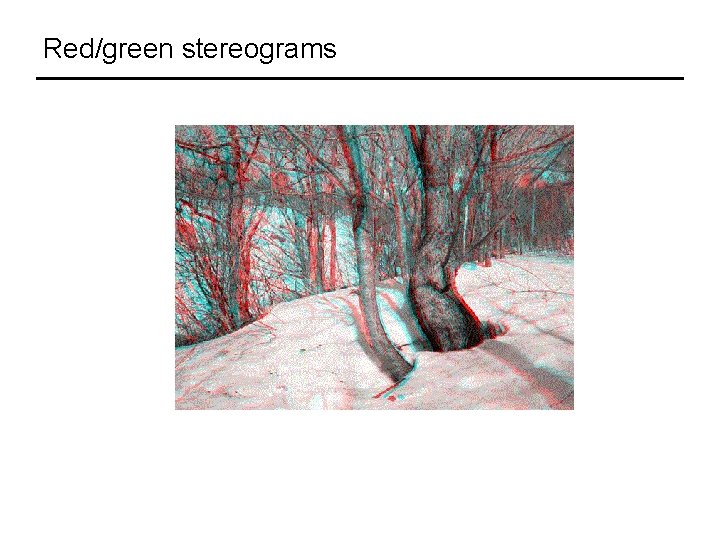
Red/green stereograms

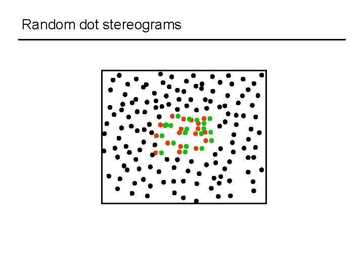
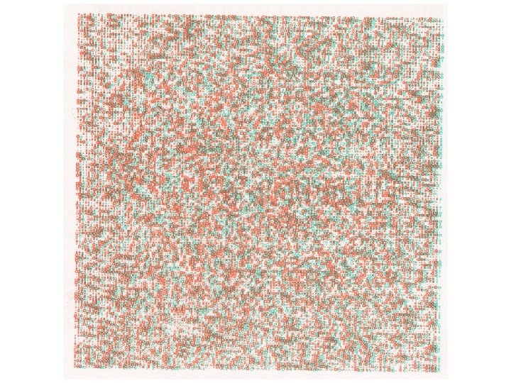
Random dot stereograms


Autostereograms: www. magiceye. com

Autostereograms: www. magiceye. com

Correspondence algorithms Algorithms may be top down or bottom up – random dot stereograms are an existence proof that bottom up algorithms are possible From here on only consider bottom up algorithms Algorithms may be classified into two types: 1. Dense: compute a correspondence at every pixel 2. Sparse: compute correspondences only for features

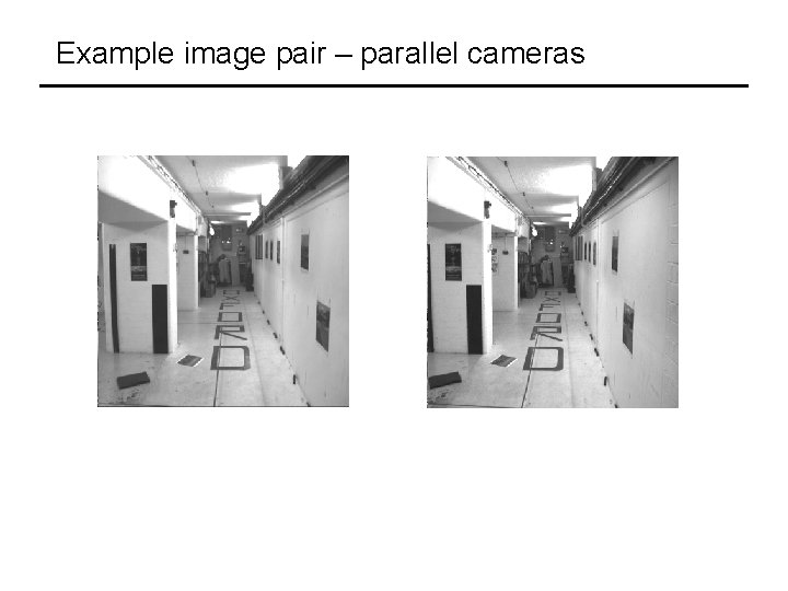
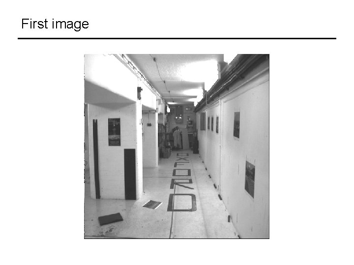
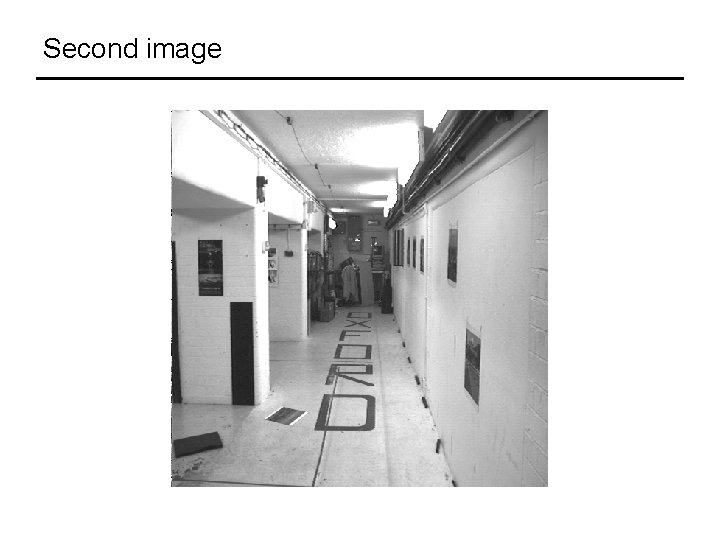
Example image pair – parallel cameras

First image

Second image

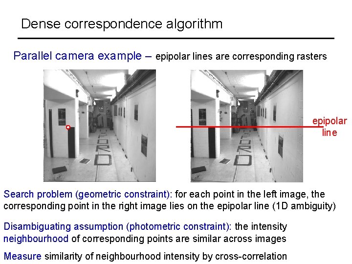
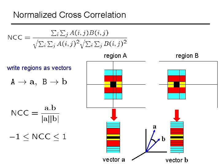
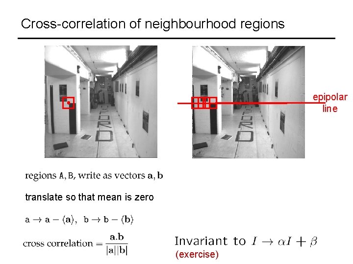
Dense correspondence algorithm Parallel camera example – epipolar lines are corresponding rasters epipolar line Search problem (geometric constraint): for each point in the left image, the corresponding point in the right image lies on the epipolar line (1 D ambiguity) Disambiguating assumption (photometric constraint): the intensity neighbourhood of corresponding points are similar across images Measure similarity of neighbourhood intensity by cross-correlation

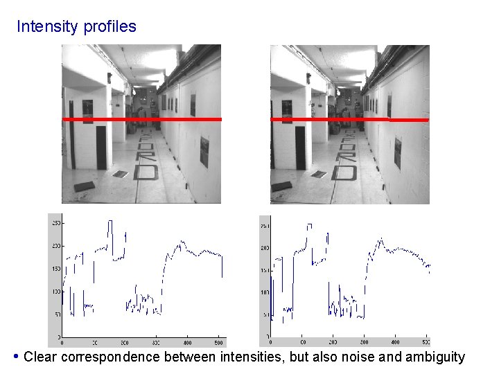
Intensity profiles • Clear correspondence between intensities, but also noise and ambiguity

Normalized Cross Correlation region A region B write regions as vectors a b vector a vector b

Cross-correlation of neighbourhood regions epipolar line translate so that mean is zero (exercise)

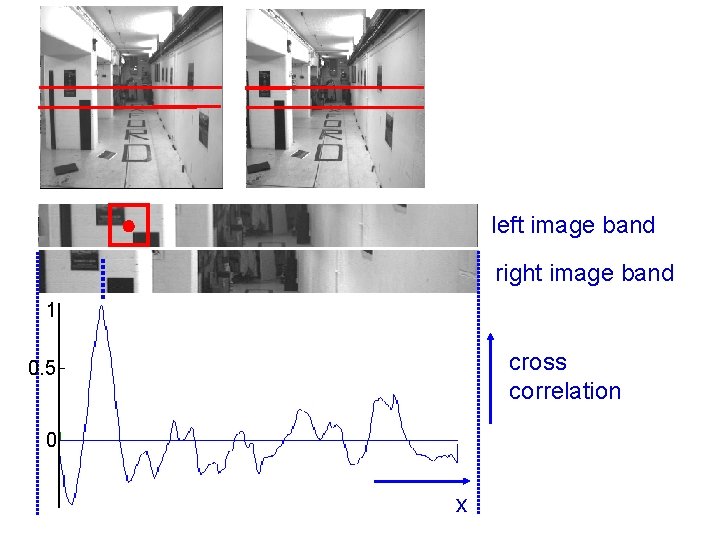
left image band right image band 1 cross correlation 0. 5 0 x

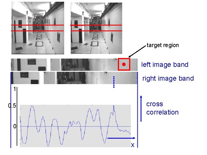
target region left image band right image band 1 cross correlation 0. 5 0 x

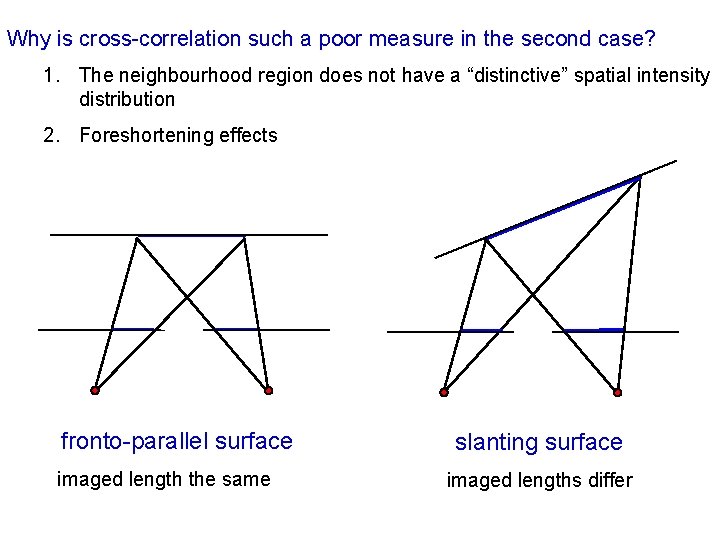
Why is cross-correlation such a poor measure in the second case? 1. The neighbourhood region does not have a “distinctive” spatial intensity distribution 2. Foreshortening effects fronto-parallel surface imaged length the same slanting surface imaged lengths differ

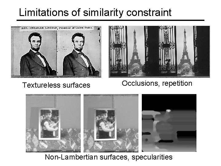
Limitations of similarity constraint Textureless surfaces Occlusions, repetition Non-Lambertian surfaces, specularities

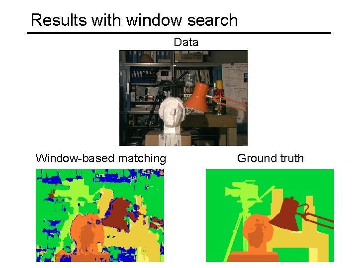
Results with window search Data Window-based matching Ground truth

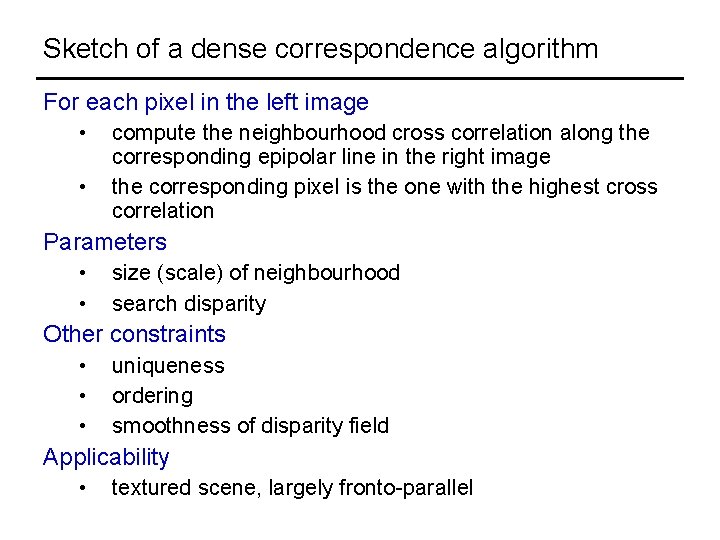
Sketch of a dense correspondence algorithm For each pixel in the left image • • compute the neighbourhood cross correlation along the corresponding epipolar line in the right image the corresponding pixel is the one with the highest cross correlation Parameters • • size (scale) of neighbourhood search disparity Other constraints • • • uniqueness ordering smoothness of disparity field Applicability • textured scene, largely fronto-parallel

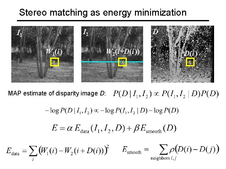
Stereo matching as energy minimization I 2 I 1 W 1(i ) D W 2(i+D(i )) MAP estimate of disparity image D: D(i )

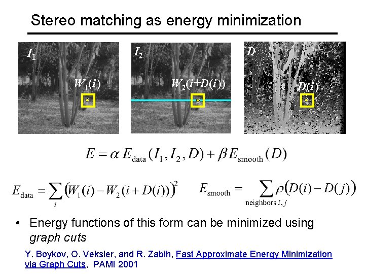
Stereo matching as energy minimization I 2 I 1 W 1(i ) D W 2(i+D(i )) D(i ) • Energy functions of this form can be minimized using graph cuts Y. Boykov, O. Veksler, and R. Zabih, Fast Approximate Energy Minimization via Graph Cuts, PAMI 2001

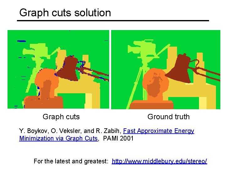
Graph cuts solution Graph cuts Ground truth Y. Boykov, O. Veksler, and R. Zabih, Fast Approximate Energy Minimization via Graph Cuts, PAMI 2001 For the latest and greatest: http: //www. middlebury. edu/stereo/

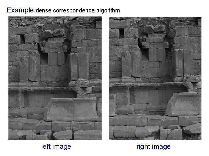
Example dense correspondence algorithm left image right image

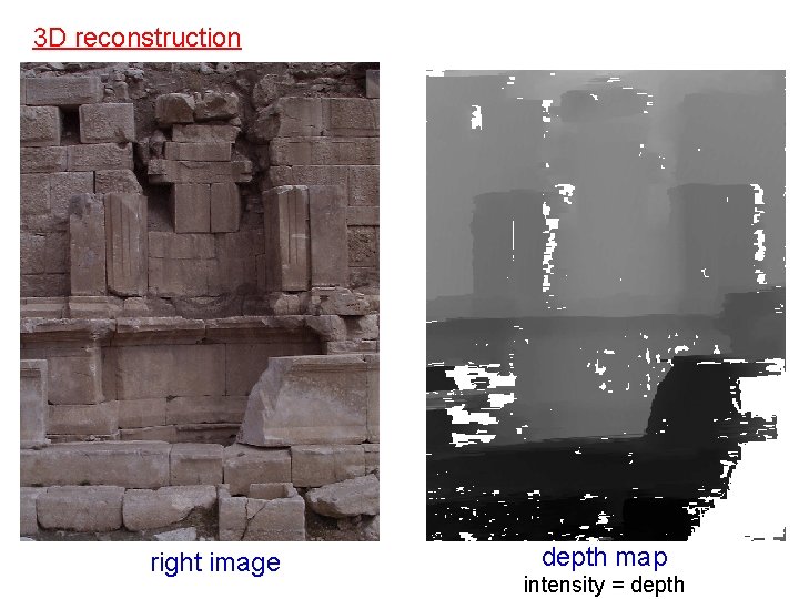
3 D reconstruction right image depth map intensity = depth

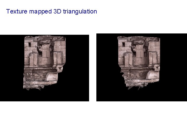
Texture mapped 3 D triangulation

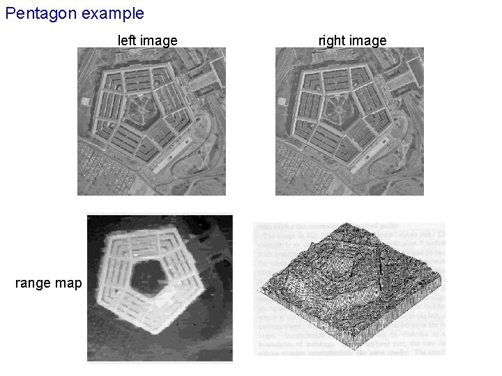
Pentagon example left image range map right image

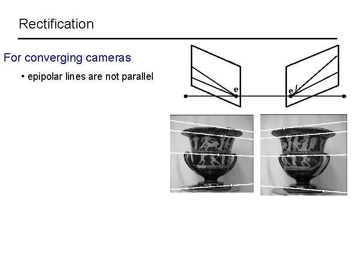
Rectification For converging cameras • epipolar lines are not parallel e e/

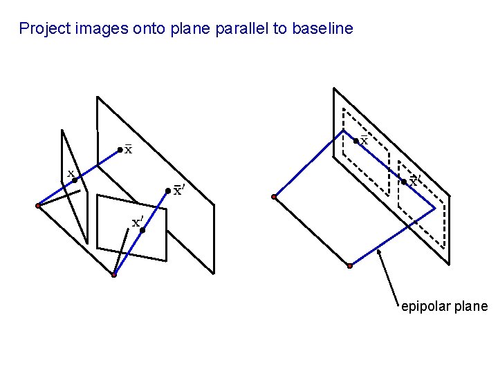
Project images onto plane parallel to baseline epipolar plane

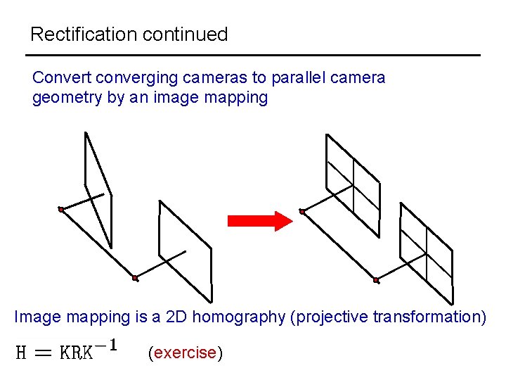
Rectification continued Convert converging cameras to parallel camera geometry by an image mapping Image mapping is a 2 D homography (projective transformation) (exercise)

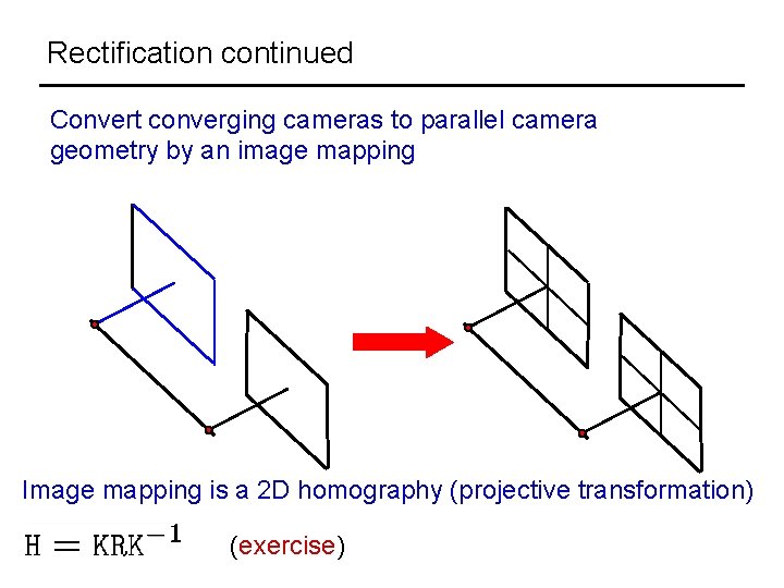
Rectification continued Convert converging cameras to parallel camera geometry by an image mapping Image mapping is a 2 D homography (projective transformation) (exercise)

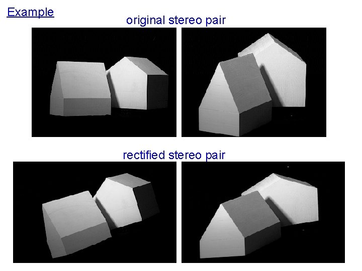
Example original stereo pair rectified stereo pair

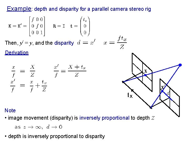
Example: depth and disparity for a parallel camera stereo rig Then, y/ = y, and the disparity Derivation x x/ Note • image movement (disparity) is inversely proportional to depth Z • depth is inversely proportional to disparity d

Triangulation

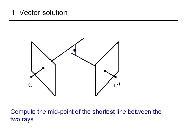
1. Vector solution C C/ Compute the mid-point of the shortest line between the two rays

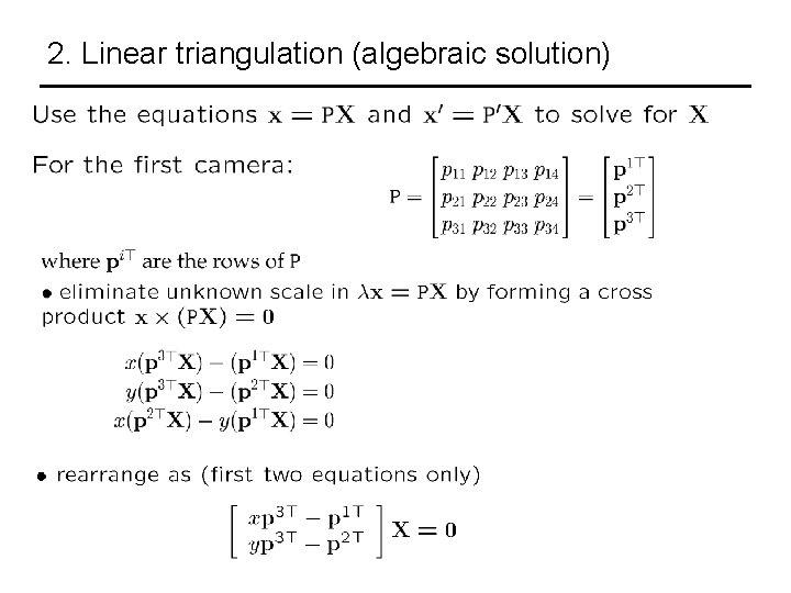
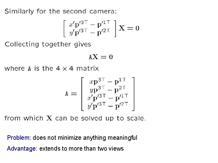
2. Linear triangulation (algebraic solution)

Problem: does not minimize anything meaningful Advantage: extends to more than two views

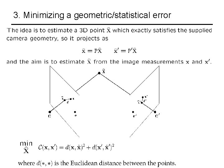
3. Minimizing a geometric/statistical error

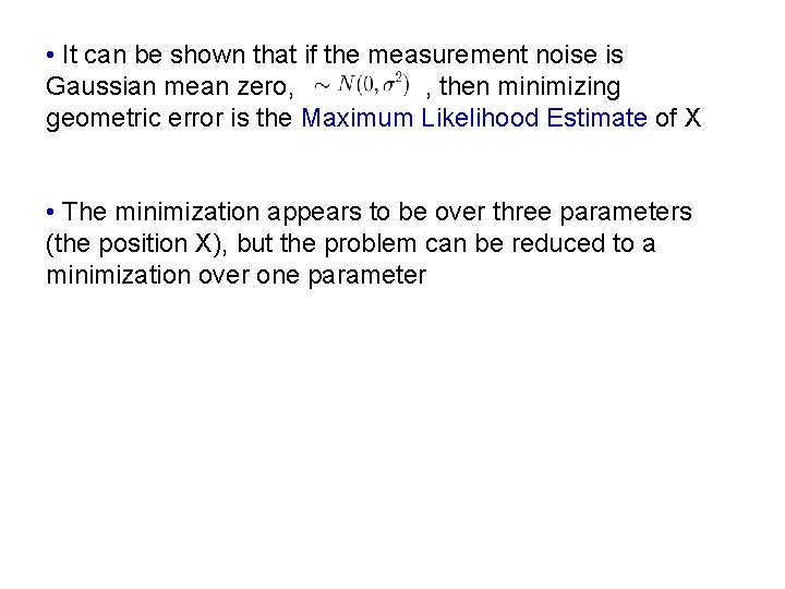
• It can be shown that if the measurement noise is Gaussian mean zero, , then minimizing geometric error is the Maximum Likelihood Estimate of X • The minimization appears to be over three parameters (the position X), but the problem can be reduced to a minimization over one parameter

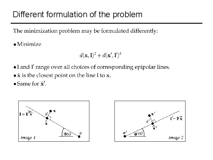
Different formulation of the problem

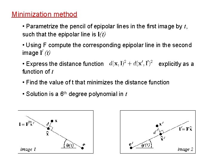
Minimization method • Parametrize the pencil of epipolar lines in the first image by t, such that the epipolar line is l(t) • Using F compute the corresponding epipolar line in the second image l/ (t) • Express the distance function of t explicitly as a • Find the value of t that minimizes the distance function • Solution is a 6 th degree polynomial in t

Other approaches to obtaining 3 D structure

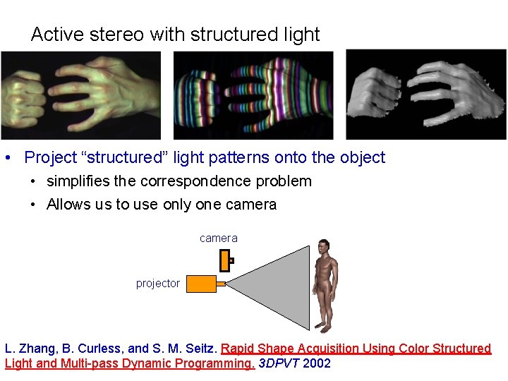
Active stereo with structured light • Project “structured” light patterns onto the object • simplifies the correspondence problem • Allows us to use only one camera projector L. Zhang, B. Curless, and S. M. Seitz. Rapid Shape Acquisition Using Color Structured Light and Multi-pass Dynamic Programming. 3 DPVT 2002

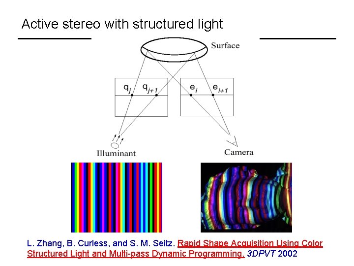
Active stereo with structured light L. Zhang, B. Curless, and S. M. Seitz. Rapid Shape Acquisition Using Color Structured Light and Multi-pass Dynamic Programming. 3 DPVT 2002

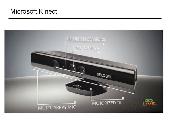
Microsoft Kinect

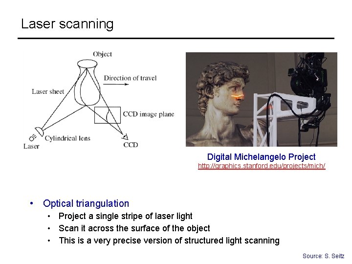
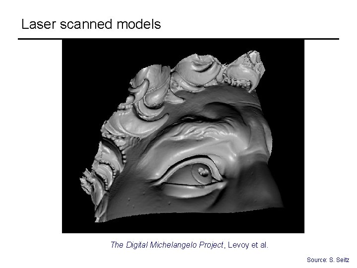
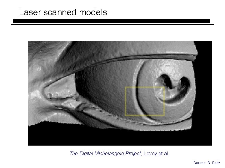
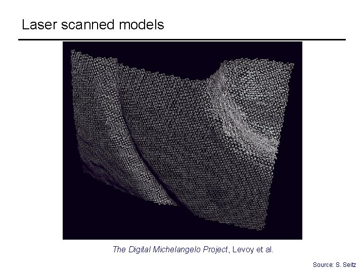
Laser scanning Digital Michelangelo Project http: //graphics. stanford. edu/projects/mich/ • Optical triangulation • Project a single stripe of laser light • Scan it across the surface of the object • This is a very precise version of structured light scanning Source: S. Seitz

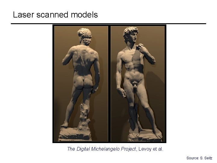
Laser scanned models The Digital Michelangelo Project, Levoy et al. Source: S. Seitz

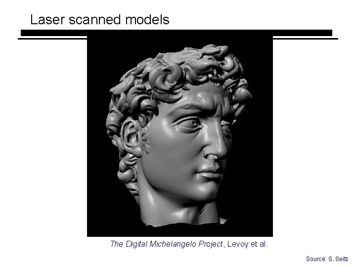
Laser scanned models The Digital Michelangelo Project, Levoy et al. Source: S. Seitz

Laser scanned models The Digital Michelangelo Project, Levoy et al. Source: S. Seitz

Laser scanned models The Digital Michelangelo Project, Levoy et al. Source: S. Seitz

Laser scanned models The Digital Michelangelo Project, Levoy et al. Source: S. Seitz

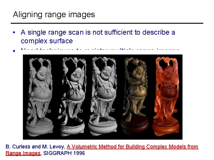
Aligning range images • A single range scan is not sufficient to describe a complex surface • Need techniques to register multiple range images B. Curless and M. Levoy, A Volumetric Method for Building Complex Models from Range Images, SIGGRAPH 1996

Aligning range images • A single range scan is not sufficient to describe a complex surface • Need techniques to register multiple range images • … which brings us to multi-view stereo