3 DIFFERENTIATION RULES DIFFERENTIATION RULES 3 8 Exponential

3 DIFFERENTIATION RULES

DIFFERENTIATION RULES 3. 8 Exponential Growth and Decay In this section, we will: Use differentiation to solve real-life problems involving exponentially growing quantities.

EXPONENTIAL GROWTH & DECAY In many natural phenomena, quantities grow or decay at a rate proportional to their size.

EXAMPLE For instance, suppose y = f(t) is the number of individuals in a population of animals or bacteria at time t. § Then, it seems reasonable to expect that the rate of growth f’(t) is proportional to the population f(t). § That is, f’(t) = kf(t) for some constant k.

EXPONENTIAL GROWTH & DECAY Indeed, under ideal conditions—unlimited environment, adequate nutrition, and immunity to disease—the mathematical model given by the equation f’(t) = kf(t) predicts what actually happens fairly accurately.

EXAMPLE Another example occurs in nuclear physics where the mass of a radioactive substance decays at a rate proportional to the mass.

EXAMPLE In chemistry, the rate of a unimolecular first-order reaction is proportional to the concentration of the substance.

EXAMPLE In finance, the value of a savings account with continuously compounded interest increases at a rate proportional to that value.

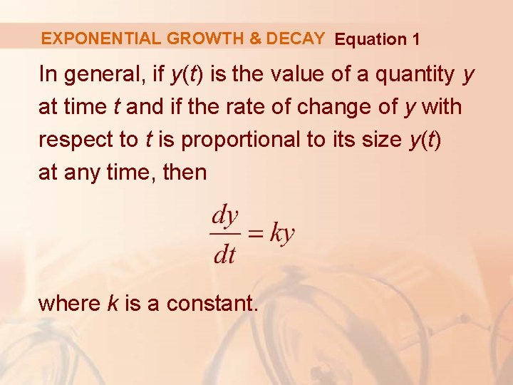
EXPONENTIAL GROWTH & DECAY Equation 1 In general, if y(t) is the value of a quantity y at time t and if the rate of change of y with respect to t is proportional to its size y(t) at any time, then where k is a constant.

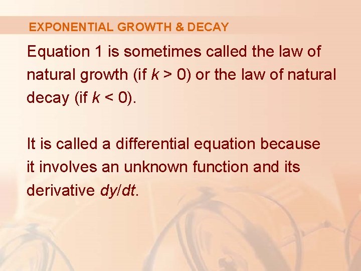
EXPONENTIAL GROWTH & DECAY Equation 1 is sometimes called the law of natural growth (if k > 0) or the law of natural decay (if k < 0). It is called a differential equation because it involves an unknown function and its derivative dy/dt.

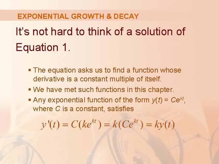
EXPONENTIAL GROWTH & DECAY It’s not hard to think of a solution of Equation 1. § The equation asks us to find a function whose derivative is a constant multiple of itself. § We have met such functions in this chapter. § Any exponential function of the form y(t) = Cekt, where C is a constant, satisfies

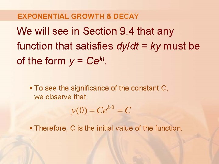
EXPONENTIAL GROWTH & DECAY We will see in Section 9. 4 that any function that satisfies dy/dt = ky must be of the form y = Cekt. § To see the significance of the constant C, we observe that § Therefore, C is the initial value of the function.

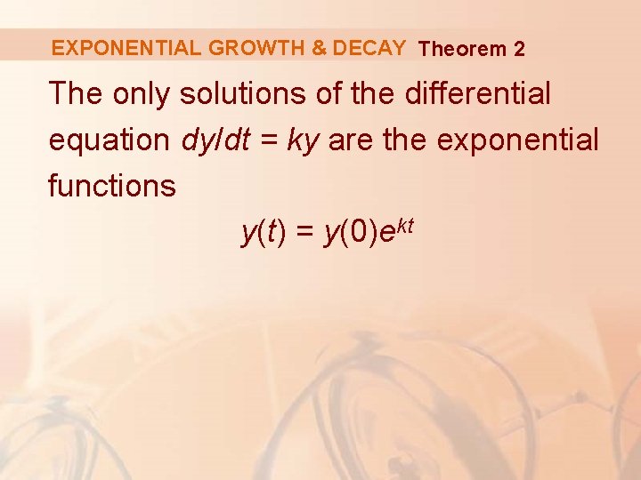
EXPONENTIAL GROWTH & DECAY Theorem 2 The only solutions of the differential equation dy/dt = ky are the exponential functions y(t) = y(0)ekt

POPULATION GROWTH What is the significance of the proportionality constant k?

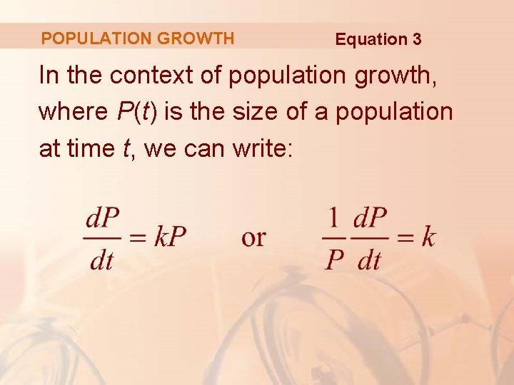
POPULATION GROWTH Equation 3 In the context of population growth, where P(t) is the size of a population at time t, we can write:

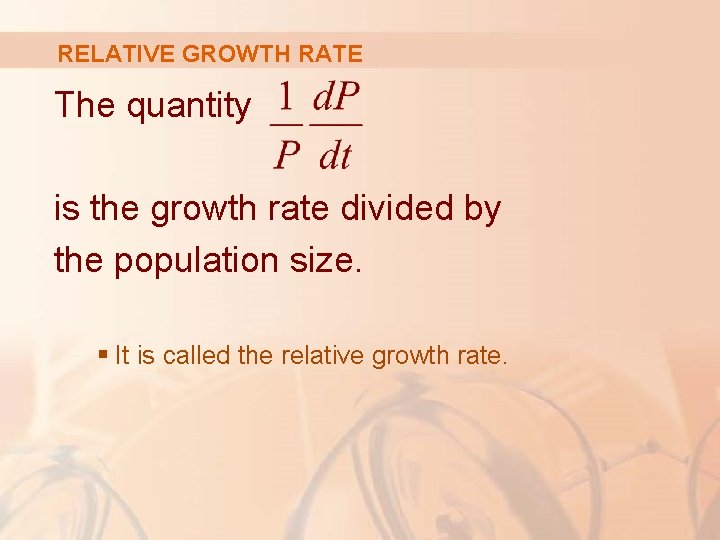
RELATIVE GROWTH RATE The quantity is the growth rate divided by the population size. § It is called the relative growth rate.

RELATIVE GROWTH RATE According to Equation 3, instead of saying “the growth rate is proportional to population size, ” we could say “the relative growth rate is constant. ” § Then, Theorem 2 states that a population with constant relative growth rate must grow exponentially.

RELATIVE GROWTH RATE Notice that the relative growth rate k appears as the coefficient of t in the exponential function Cekt.

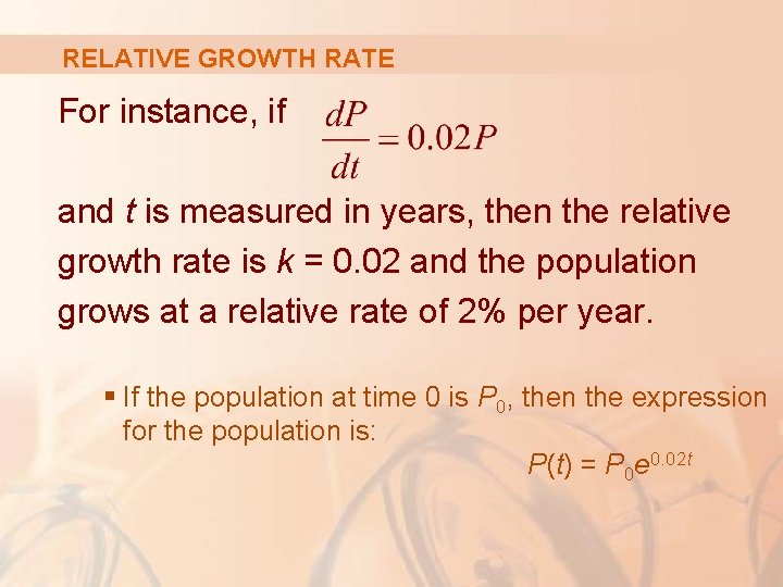
RELATIVE GROWTH RATE For instance, if and t is measured in years, then the relative growth rate is k = 0. 02 and the population grows at a relative rate of 2% per year. § If the population at time 0 is P 0, then the expression for the population is: P(t) = P 0 e 0. 02 t

POPULATION GROWTH Example 1 Use the fact that the world population was 2, 560 million in 1950 and 3, 040 million in 1960 to model the population in the second half of the 20 th century. (Assume the growth rate is proportional to the population size. ) § What is the relative growth rate? § Use the model to estimate the population in 1993 and to predict the population in 2020.

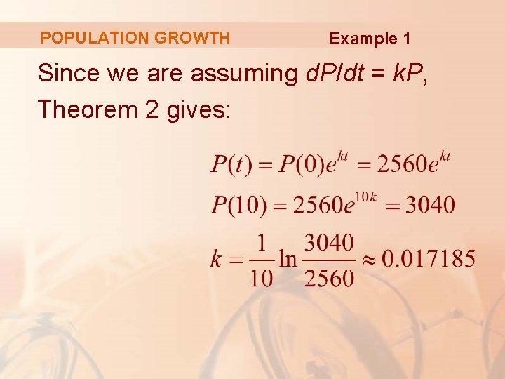
POPULATION GROWTH Example 1 We measure the time t in years and let t = 0 in 1950. We measure the population P(t) in millions of people. § Then, P(0) = 2560 and P(10) = 3040

POPULATION GROWTH Example 1 Since we are assuming d. P/dt = k. P, Theorem 2 gives:

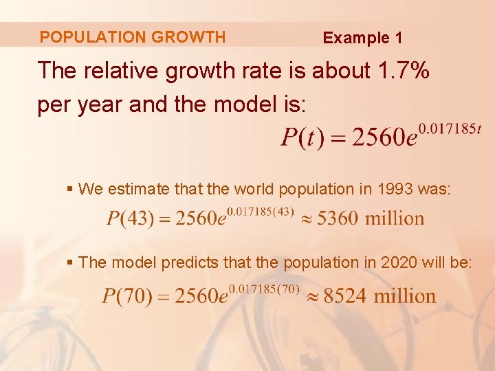
POPULATION GROWTH Example 1 The relative growth rate is about 1. 7% per year and the model is: § We estimate that the world population in 1993 was: § The model predicts that the population in 2020 will be:

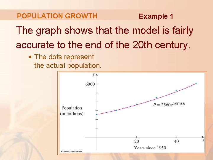
POPULATION GROWTH Example 1 The graph shows that the model is fairly accurate to the end of the 20 th century. § The dots represent the actual population.

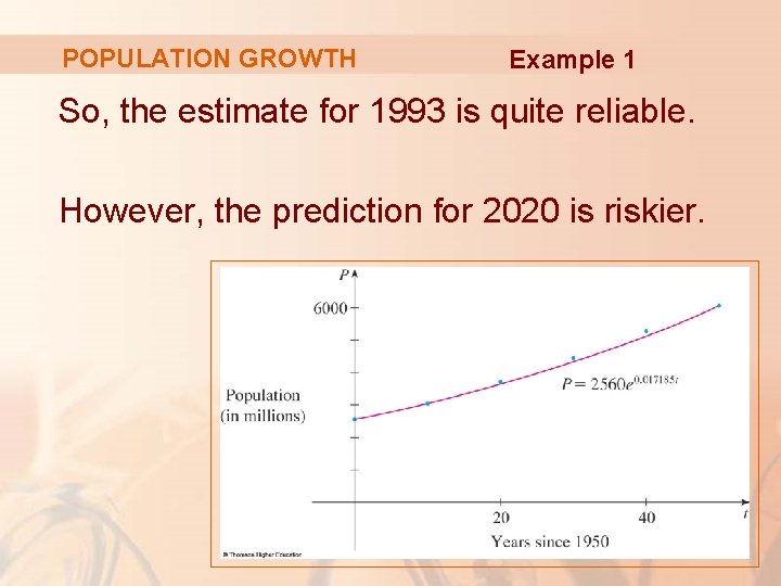
POPULATION GROWTH Example 1 So, the estimate for 1993 is quite reliable. However, the prediction for 2020 is riskier.

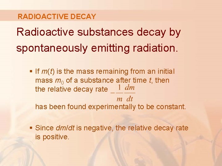
RADIOACTIVE DECAY Radioactive substances decay by spontaneously emitting radiation. § If m(t) is the mass remaining from an initial mass m 0 of a substance after time t, then the relative decay rate has been found experimentally to be constant. § Since dm/dt is negative, the relative decay rate is positive.

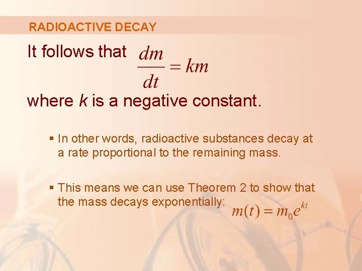
RADIOACTIVE DECAY It follows that where k is a negative constant. § In other words, radioactive substances decay at a rate proportional to the remaining mass. § This means we can use Theorem 2 to show that the mass decays exponentially:

HALF-LIFE Physicists express the rate of decay in terms of half-life. § This is the time required for half of any given quantity to decay.

RADIOACTIVE DECAY Example 2 The half-life of radium-226 is 1590 years. a. A sample of radium-226 has a mass of 100 mg. Find a formula for the mass of the sample that remains after t years. b. Find the mass after 1, 000 years correct to the nearest milligram. c. When will the mass be reduced to 30 mg?

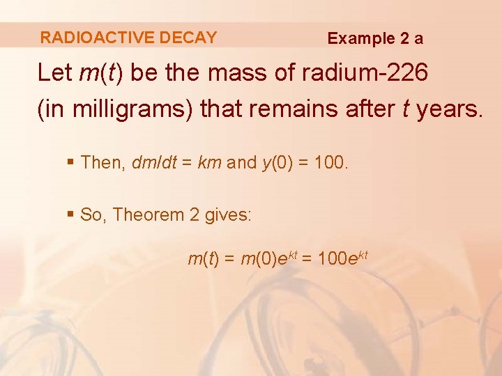
RADIOACTIVE DECAY Example 2 a Let m(t) be the mass of radium-226 (in milligrams) that remains after t years. § Then, dm/dt = km and y(0) = 100. § So, Theorem 2 gives: m(t) = m(0)ekt = 100 ekt

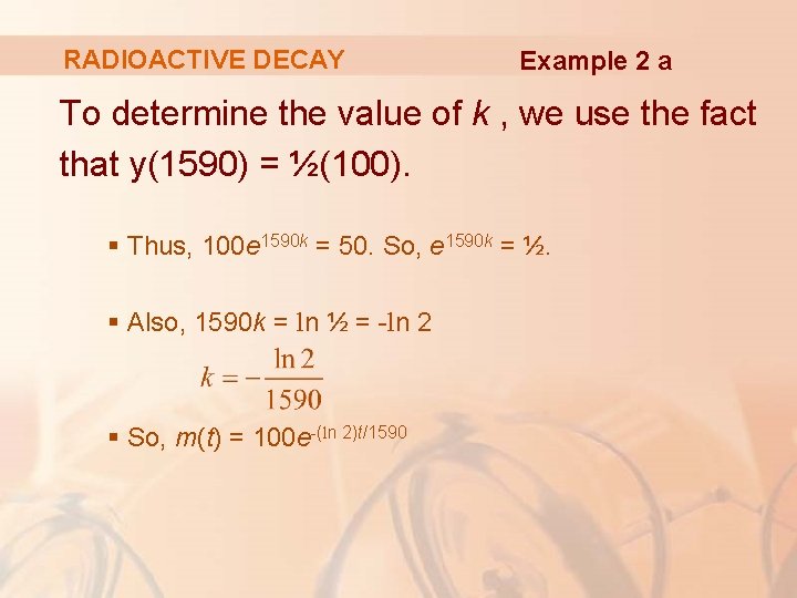
RADIOACTIVE DECAY Example 2 a To determine the value of k , we use the fact that y(1590) = ½(100). § Thus, 100 e 1590 k = 50. So, e 1590 k = ½. § Also, 1590 k = ln ½ = -ln 2 § So, m(t) = 100 e-(ln 2)t/1590

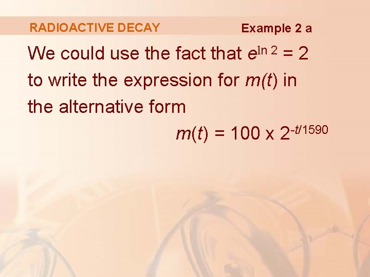
RADIOACTIVE DECAY Example 2 a We could use the fact that eln 2 = 2 to write the expression for m(t) in the alternative form m(t) = 100 x 2 -t/1590

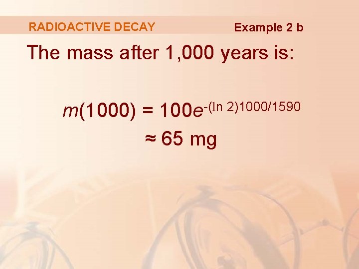
RADIOACTIVE DECAY Example 2 b The mass after 1, 000 years is: m(1000) = 100 e-(ln 2)1000/1590 ≈ 65 mg

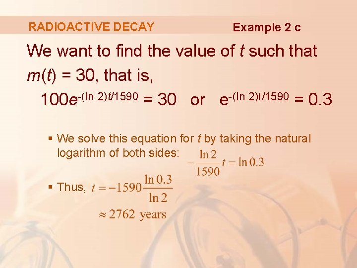
RADIOACTIVE DECAY Example 2 c We want to find the value of t such that m(t) = 30, that is, 100 e-(ln 2)t/1590 = 30 or e-(ln 2)t/1590 = 0. 3 § We solve this equation for t by taking the natural logarithm of both sides: § Thus,

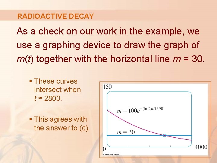
RADIOACTIVE DECAY As a check on our work in the example, we use a graphing device to draw the graph of m(t) together with the horizontal line m = 30. § These curves intersect when t ≈ 2800. § This agrees with the answer to (c).

NEWTON’S LAW OF COOLING Newton’s Law of Cooling states: The rate of cooling of an object is proportional to the temperature difference between the object and its surroundings—provided the difference is not too large. § The law also applies to warming.

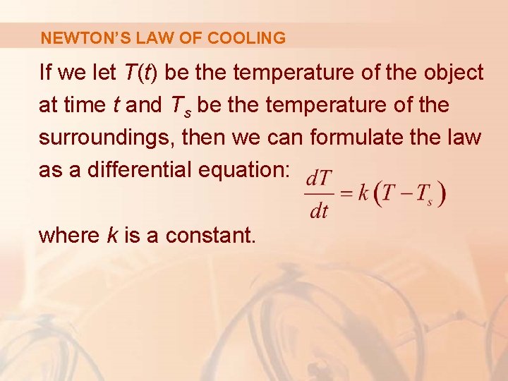
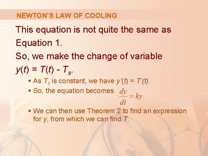
NEWTON’S LAW OF COOLING If we let T(t) be the temperature of the object at time t and Ts be the temperature of the surroundings, then we can formulate the law as a differential equation: where k is a constant.

NEWTON’S LAW OF COOLING This equation is not quite the same as Equation 1. So, we make the change of variable y(t) = T(t) - Ts. § As Ts is constant, we have y’(t) = T’(t). § So, the equation becomes § We can then use Theorem 2 to find an expression for y, from which we can find T.

NEWTON’S LAW OF COOLING Example 3 A bottle of soda pop at room temperature (72°F) is placed in a refrigerator, where the temperature is 44°F. After half an hour, the soda pop has cooled to 61°F. a) What is the temperature of the soda pop after another half hour? b) How long does it take for the soda pop to cool to 50°F?

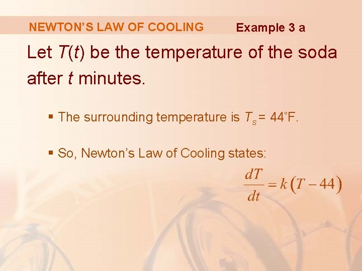
NEWTON’S LAW OF COOLING Example 3 a Let T(t) be the temperature of the soda after t minutes. § The surrounding temperature is Ts = 44°F. § So, Newton’s Law of Cooling states:

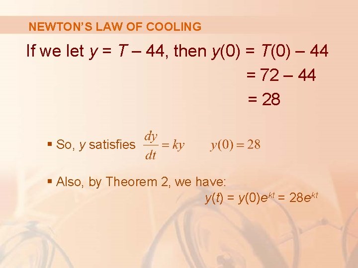
NEWTON’S LAW OF COOLING If we let y = T – 44, then y(0) = T(0) – 44 = 72 – 44 = 28 § So, y satisfies § Also, by Theorem 2, we have: y(t) = y(0)ekt = 28 ekt

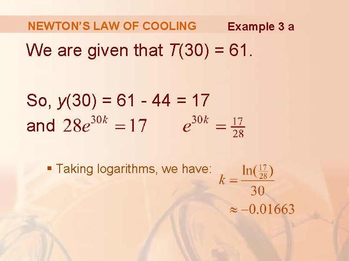
NEWTON’S LAW OF COOLING Example 3 a We are given that T(30) = 61. So, y(30) = 61 - 44 = 17 and § Taking logarithms, we have:

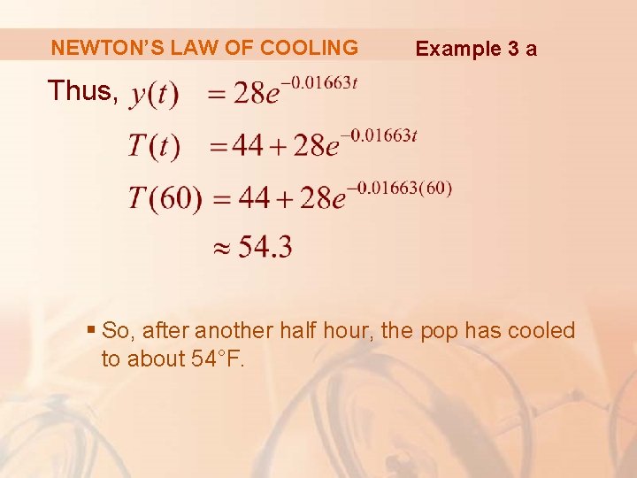
NEWTON’S LAW OF COOLING Example 3 a Thus, § So, after another half hour, the pop has cooled to about 54°F.

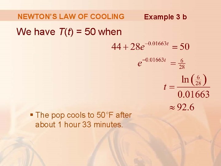
NEWTON’S LAW OF COOLING We have T(t) = 50 when § The pop cools to 50°F after about 1 hour 33 minutes. Example 3 b

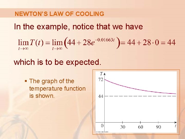
NEWTON’S LAW OF COOLING In the example, notice that we have which is to be expected. § The graph of the temperature function is shown.

EXPONENTIAL GROWTH & DECAY Finally, we will look at an example of continuously compounded interest.

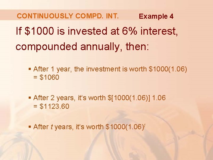
CONTINUOUSLY COMPD. INT. Example 4 If $1000 is invested at 6% interest, compounded annually, then: § After 1 year, the investment is worth $1000(1. 06) = $1060 § After 2 years, it’s worth $[1000(1. 06)] 1. 06 = $1123. 60 § After t years, it’s worth $1000(1. 06)t

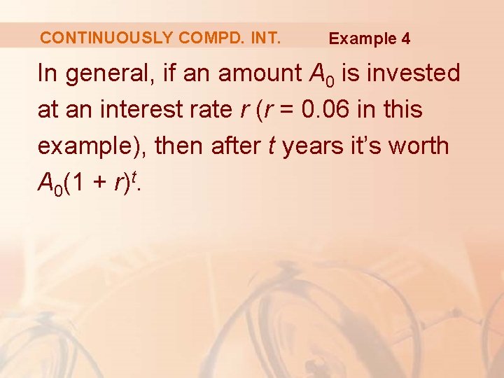
CONTINUOUSLY COMPD. INT. Example 4 In general, if an amount A 0 is invested at an interest rate r (r = 0. 06 in this example), then after t years it’s worth A 0(1 + r)t.

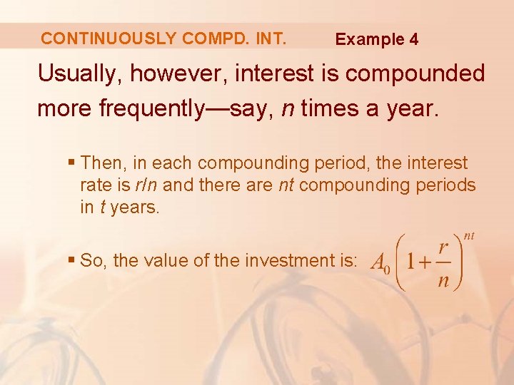
CONTINUOUSLY COMPD. INT. Example 4 Usually, however, interest is compounded more frequently—say, n times a year. § Then, in each compounding period, the interest rate is r/n and there are nt compounding periods in t years. § So, the value of the investment is:

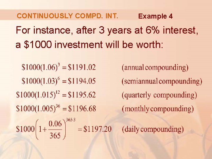
CONTINUOUSLY COMPD. INT. Example 4 For instance, after 3 years at 6% interest, a $1000 investment will be worth:

CONTINUOUSLY COMPD. INT. Example 4 You can see that the interest paid increases as the number of compounding periods (n) increases.

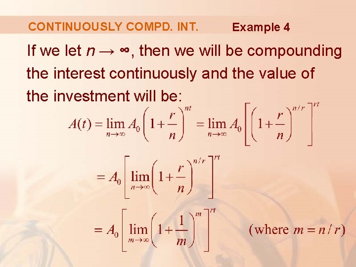
CONTINUOUSLY COMPD. INT. Example 4 If we let n → ∞, then we will be compounding the interest continuously and the value of the investment will be:

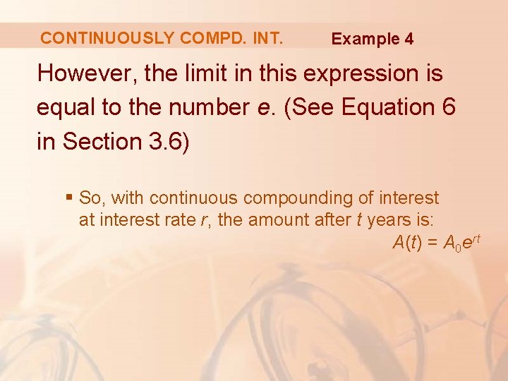
CONTINUOUSLY COMPD. INT. Example 4 However, the limit in this expression is equal to the number e. (See Equation 6 in Section 3. 6) § So, with continuous compounding of interest at interest rate r, the amount after t years is: A(t) = A 0 ert

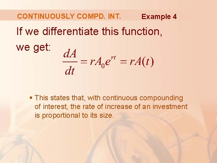
CONTINUOUSLY COMPD. INT. Example 4 If we differentiate this function, we get: § This states that, with continuous compounding of interest, the rate of increase of an investment is proportional to its size.

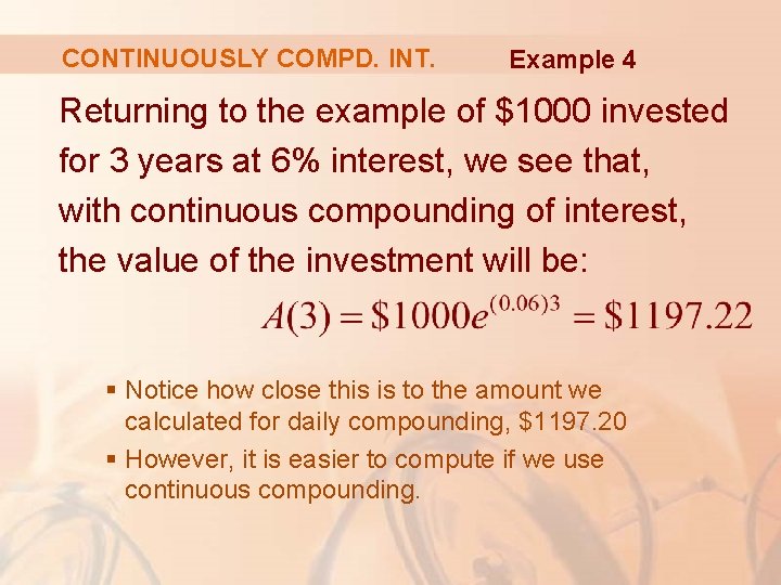
CONTINUOUSLY COMPD. INT. Example 4 Returning to the example of $1000 invested for 3 years at 6% interest, we see that, with continuous compounding of interest, the value of the investment will be: § Notice how close this is to the amount we calculated for daily compounding, $1197. 20 § However, it is easier to compute if we use continuous compounding.