12 Managing Uncertainty in a Supply Chain Safety

12 Managing Uncertainty in a Supply Chain: Safety Inventory Power. Point presentation to accompany Chopra and Meindl Supply Chain Management, 5 e Global Edition Copyright © 2013 Pearson Education. 12 -1 1 -1

Learning Objectives 1. Understand the role of safety inventory in a supply chain 2. Identify factors that influence the required level of safety inventory 3. Describe different measures of product availability 4. Determine the appropriate level of safety inventory 5. Impact of supply uncertainty on safety inventory 6. Impact of aggregation on safety inventory 7. Impact of replenishment policies on safety inventory 8. Utilize managerial levers available to lower safety inventory and improve product availability Copyright © 2013 Pearson Education. 12 -2

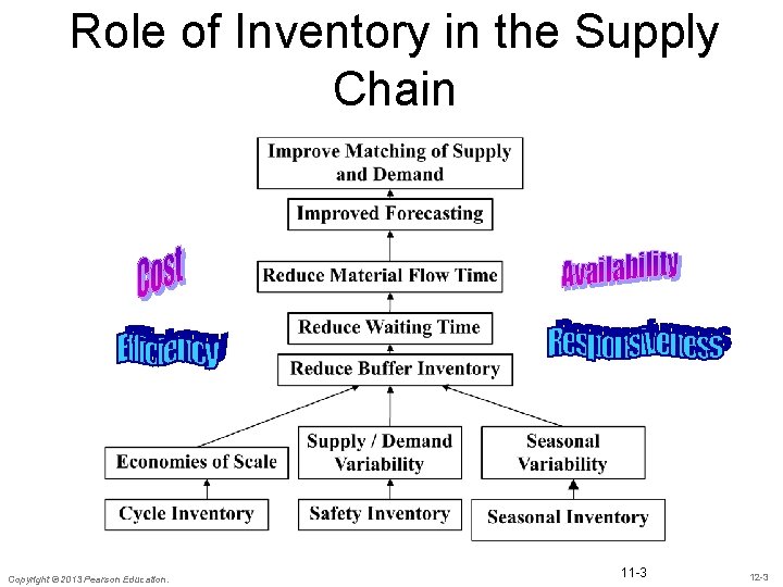
Role of Inventory in the Supply Chain Copyright © 2013 Pearson Education. 11 -3 12 -3

The Role of Safety Inventory in a Supply Chain u Forecasts are rarely completely accurate u If average demand is 1000 units per week, then half the time actual demand will be greater than 1000, and half the time actual demand will be less than 1000; what happens when actual demand is greater than 1000? u If you kept only enough inventory in stock to satisfy average demand, half the time you would run out u Safety inventory: Inventory carried for the purpose of satisfying demand that exceeds the amount forecasted in a given period Copyright © 2010 Pearson Education, Inc. Publishing as Prentice Hall. 11 -4

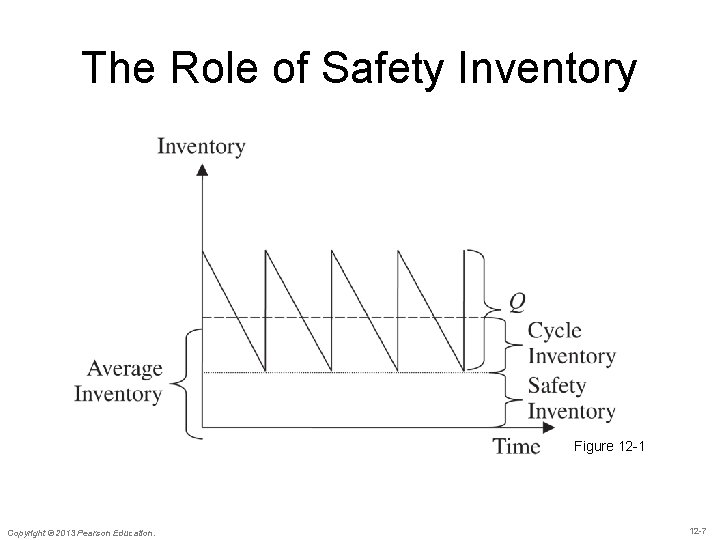
Role of Safety Inventory u. Average inventory is therefore cycle inventory plus safety inventory u. There is a fundamental tradeoff: – Raising the level of safety inventory provides higher levels of product availability and customer service, and thus the margin captured from customer purchases – Raising the level of safety inventory also raises the level of average inventory and therefore increases holding costs » Very important in high-tech or other industries where obsolescence is a significant risk (where the value of inventory, such as PCs, can drop in value) Copyright © 2010 Pearson Education, Inc. Publishing as Prentice Hall. 11 -5

The Role of Safety Inventory • Three key questions 1. What is the appropriate level of product availability? 2. How much safety inventory is needed for the desired level of product availability? 3. What actions can be taken to improve product availability while reducing safety inventory? Copyright © 2013 Pearson Education. 12 -6

The Role of Safety Inventory Figure 12 -1 Copyright © 2013 Pearson Education. 12 -7

Determining the Appropriate Level of Safety Inventory u. Measuring demand uncertainty u. Measuring product availability u. Replenishment policies u. Evaluating cycle service level and fill rate u. Evaluating safety level given desired cycle service level or fill rate u. Impact of required product availability and uncertainty on safety inventory Copyright © 2010 Pearson Education, Inc. Publishing as Prentice Hall. 11 -8

Determining the Appropriate Level of Demand Uncertainty u. Appropriate level of safety inventory determined by: – supply or demand uncertainty – desired level of product availability u. Higher levels of uncertainty require higher levels of safety inventory given a particular desired level of product availability u. Higher levels of desired product availability require higher levels of safety inventory given a particular level of uncertainty Copyright © 2010 Pearson Education, Inc. Publishing as Prentice Hall. 11 -9

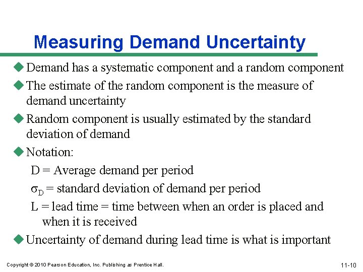
Measuring Demand Uncertainty u Demand has a systematic component and a random component u The estimate of the random component is the measure of demand uncertainty u Random component is usually estimated by the standard deviation of demand u Notation: D = Average demand period D = standard deviation of demand period L = lead time = time between when an order is placed and when it is received u Uncertainty of demand during lead time is what is important Copyright © 2010 Pearson Education, Inc. Publishing as Prentice Hall. 11 -10

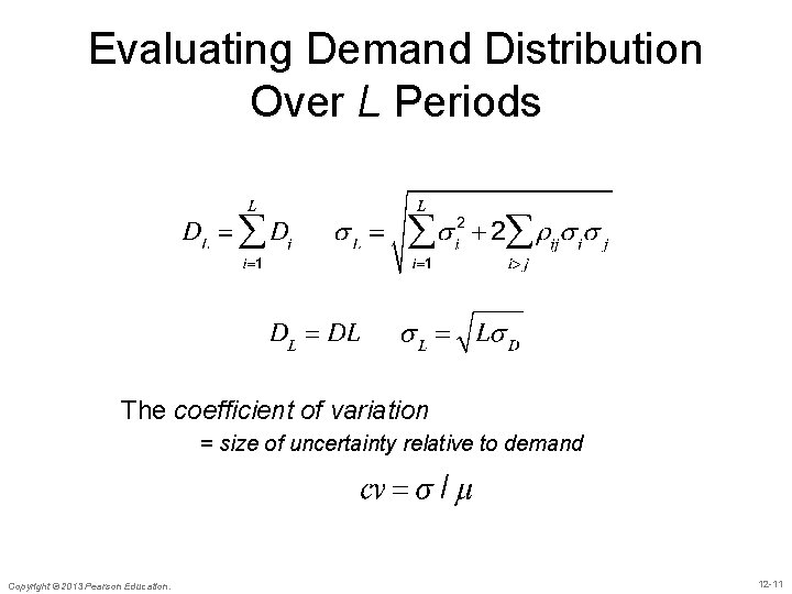
Evaluating Demand Distribution Over L Periods The coefficient of variation = size of uncertainty relative to demand Copyright © 2013 Pearson Education. 12 -11

Measuring Product Availability Ø Product availability: a firm’s ability to fill a customer’s order out of available inventory Ø Stockout: a customer order arrives when product is not available u. Product fill rate (fr): fraction of demand that is satisfied from product in inventory u. Order fill rate: fraction of orders that are filled from available inventory u. Cycle service level (CSL): fraction of replenishment cycles that end with all customer demand met Copyright © 2010 Pearson Education, Inc. Publishing as Prentice Hall. 11 -12

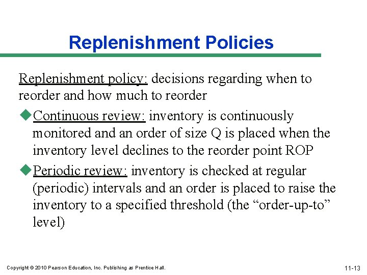
Replenishment Policies Replenishment policy: decisions regarding when to reorder and how much to reorder u. Continuous review: inventory is continuously monitored an order of size Q is placed when the inventory level declines to the reorder point ROP u. Periodic review: inventory is checked at regular (periodic) intervals and an order is placed to raise the inventory to a specified threshold (the “order-up-to” level) Copyright © 2010 Pearson Education, Inc. Publishing as Prentice Hall. 11 -13

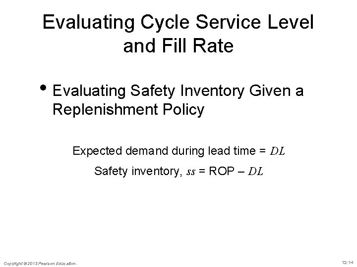
Evaluating Cycle Service Level and Fill Rate • Evaluating Safety Inventory Given a Replenishment Policy Expected demand during lead time = DL Safety inventory, ss = ROP – DL Copyright © 2013 Pearson Education. 12 -14

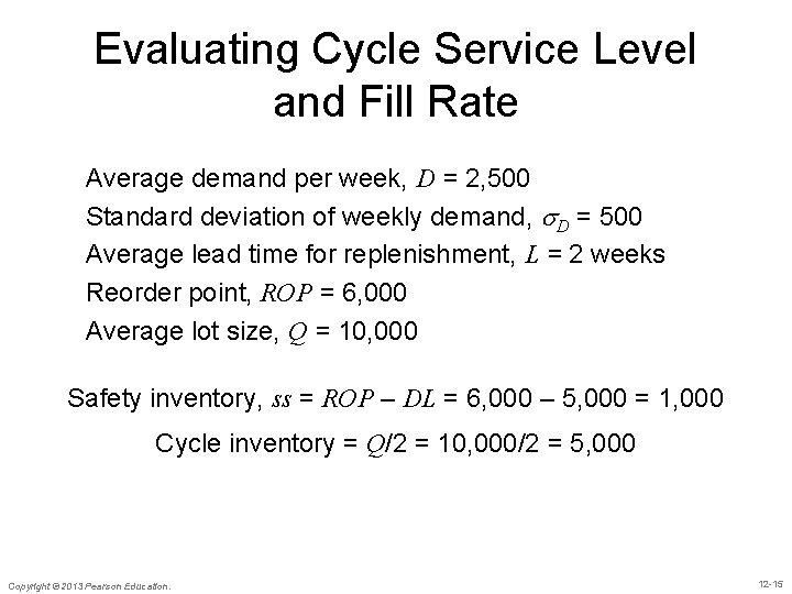
Evaluating Cycle Service Level and Fill Rate Average demand per week, D = 2, 500 Standard deviation of weekly demand, D = 500 Average lead time for replenishment, L = 2 weeks Reorder point, ROP = 6, 000 Average lot size, Q = 10, 000 Safety inventory, ss = ROP – DL = 6, 000 – 5, 000 = 1, 000 Cycle inventory = Q/2 = 10, 000/2 = 5, 000 Copyright © 2013 Pearson Education. 12 -15

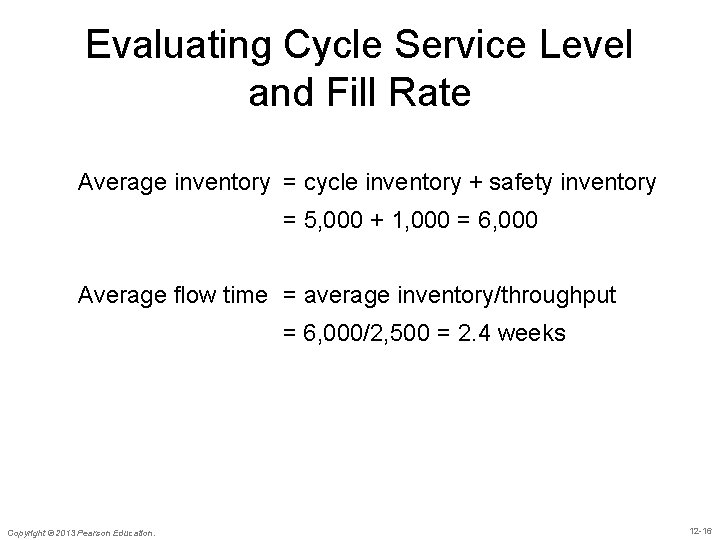
Evaluating Cycle Service Level and Fill Rate Average inventory = cycle inventory + safety inventory = 5, 000 + 1, 000 = 6, 000 Average flow time = average inventory/throughput = 6, 000/2, 500 = 2. 4 weeks Copyright © 2013 Pearson Education. 12 -16

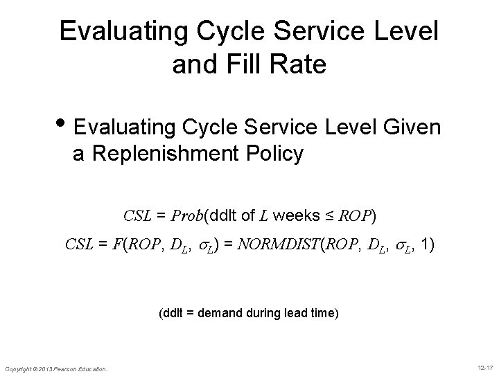
Evaluating Cycle Service Level and Fill Rate • Evaluating Cycle Service Level Given a Replenishment Policy CSL = Prob(ddlt of L weeks ≤ ROP) CSL = F(ROP, DL, L) = NORMDIST(ROP, DL, L, 1) (ddlt = demand during lead time) Copyright © 2013 Pearson Education. 12 -17

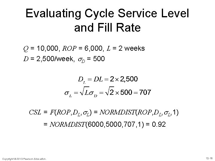
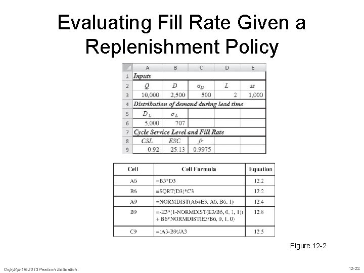
Evaluating Cycle Service Level and Fill Rate Q = 10, 000, ROP = 6, 000, L = 2 weeks D = 2, 500/week, D = 500 CSL = F(ROP, DL, L) = NORMDIST(ROP, DL, L, 1) = NORMDIST(6000, 5000, 707, 1) = 0. 92 Copyright © 2013 Pearson Education. 12 -18

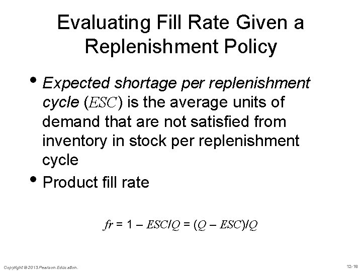
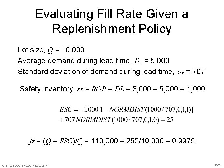
Evaluating Fill Rate Given a Replenishment Policy • Expected shortage per replenishment • cycle (ESC) is the average units of demand that are not satisfied from inventory in stock per replenishment cycle Product fill rate fr = 1 – ESC/Q = (Q – ESC)/Q Copyright © 2013 Pearson Education. 12 -19

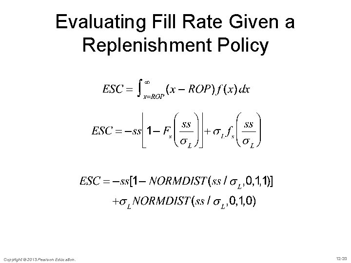
Evaluating Fill Rate Given a Replenishment Policy Copyright © 2013 Pearson Education. 12 -20

Evaluating Fill Rate Given a Replenishment Policy Lot size, Q = 10, 000 Average demand during lead time, DL = 5, 000 Standard deviation of demand during lead time, L = 707 Safety inventory, ss = ROP – DL = 6, 000 – 5, 000 = 1, 000 fr = (Q – ESC)/Q = 110, 000 – 252/10, 000 = 0. 9975 Copyright © 2013 Pearson Education. 12 -21

Evaluating Fill Rate Given a Replenishment Policy Figure 12 -2 Copyright © 2013 Pearson Education. 12 -22

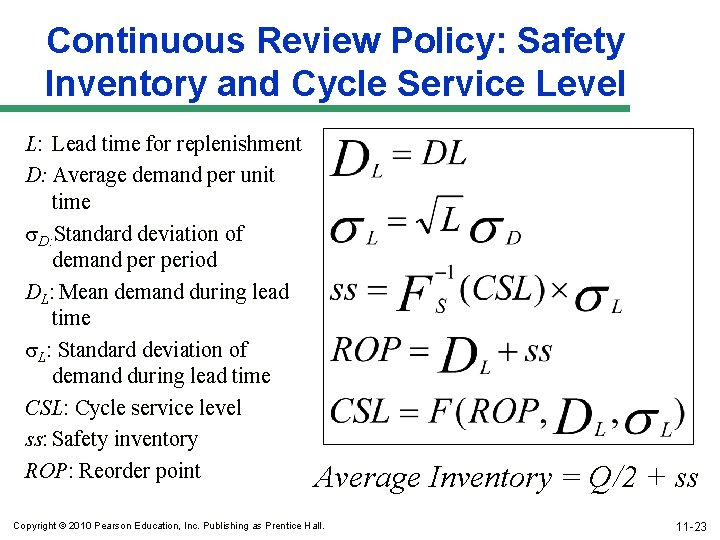
Continuous Review Policy: Safety Inventory and Cycle Service Level L: Lead time for replenishment D: Average demand per unit time D: Standard deviation of demand period DL: Mean demand during lead time L: Standard deviation of demand during lead time CSL: Cycle service level ss: Safety inventory ROP: Reorder point Average Inventory = Q/2 + ss Copyright © 2010 Pearson Education, Inc. Publishing as Prentice Hall. 11 -23

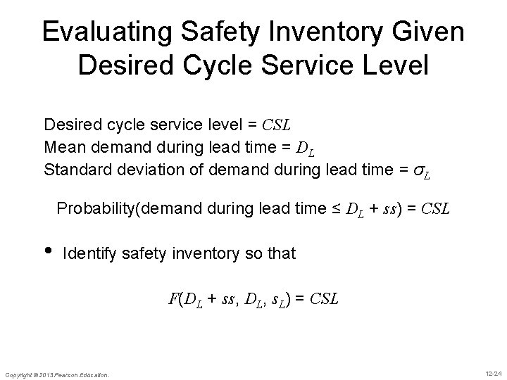
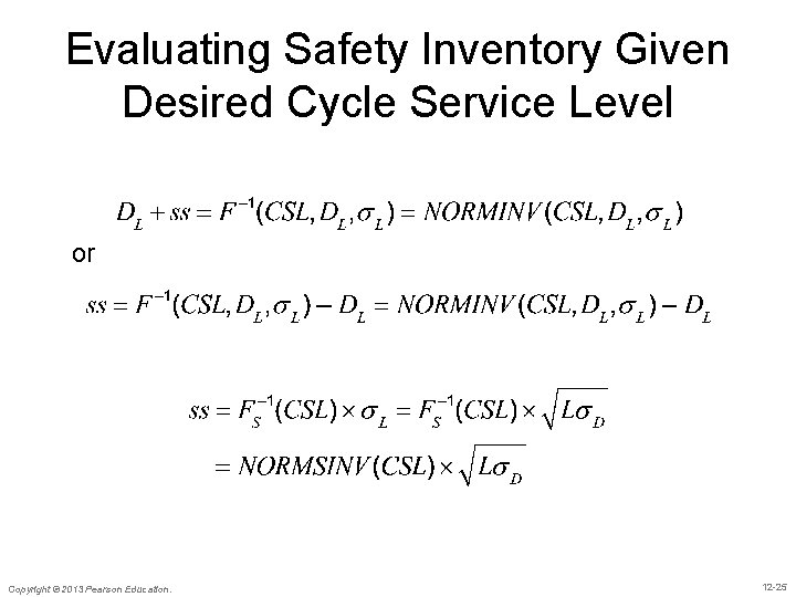
Evaluating Safety Inventory Given Desired Cycle Service Level Desired cycle service level = CSL Mean demand during lead time = DL Standard deviation of demand during lead time = σL Probability(demand during lead time ≤ DL + ss) = CSL • Identify safety inventory so that F(DL + ss, DL, s. L) = CSL Copyright © 2013 Pearson Education. 12 -24

Evaluating Safety Inventory Given Desired Cycle Service Level or Copyright © 2013 Pearson Education. 12 -25

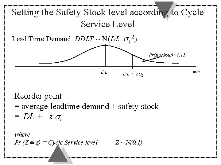
Setting the Safety Stock level according to Cycle Service Level Lead Time Demand DDLT ~ N(DL, L 2) Pr(stockout)=0. 15 DL DL + z L Reorder point = average leadtime demand + safety stock = DL + z L where Pr (Z < z) = Cycle Service level Z ~ N(0, 1) units

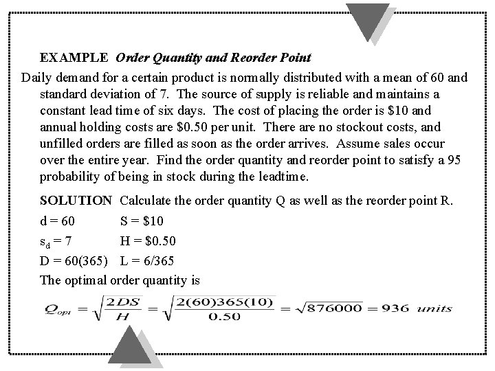
EXAMPLE Order Quantity and Reorder Point Daily demand for a certain product is normally distributed with a mean of 60 and standard deviation of 7. The source of supply is reliable and maintains a constant lead time of six days. The cost of placing the order is $10 and annual holding costs are $0. 50 per unit. There are no stockout costs, and unfilled orders are filled as soon as the order arrives. Assume sales occur over the entire year. Find the order quantity and reorder point to satisfy a 95 probability of being in stock during the leadtime. SOLUTION Calculate the order quantity Q as well as the reorder point R. d = 60 S = $10 sd = 7 H = $0. 50 D = 60(365) L = 6/365 The optimal order quantity is

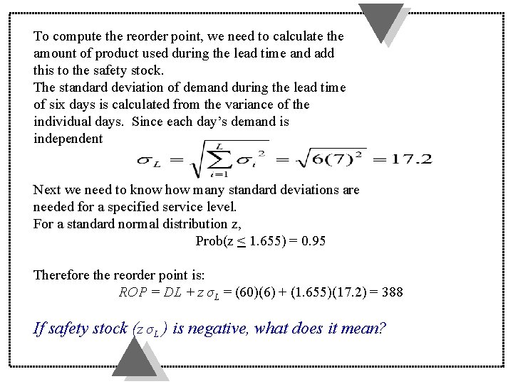
To compute the reorder point, we need to calculate the amount of product used during the lead time and add this to the safety stock. The standard deviation of demand during the lead time of six days is calculated from the variance of the individual days. Since each day’s demand is independent Next we need to know how many standard deviations are needed for a specified service level. For a standard normal distribution z, Prob(z < 1. 655) = 0. 95 Therefore the reorder point is: ROP = DL + z σL = (60)(6) + (1. 655)(17. 2) = 388 If safety stock (z σL ) is negative, what does it mean?

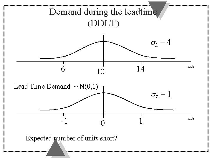
Demand during the leadtime (DDLT) L = 4 6 10 14 Lead Time Demand ~ N(0, 1) -1 units L = 1 0 Expected number of units short? 1 units

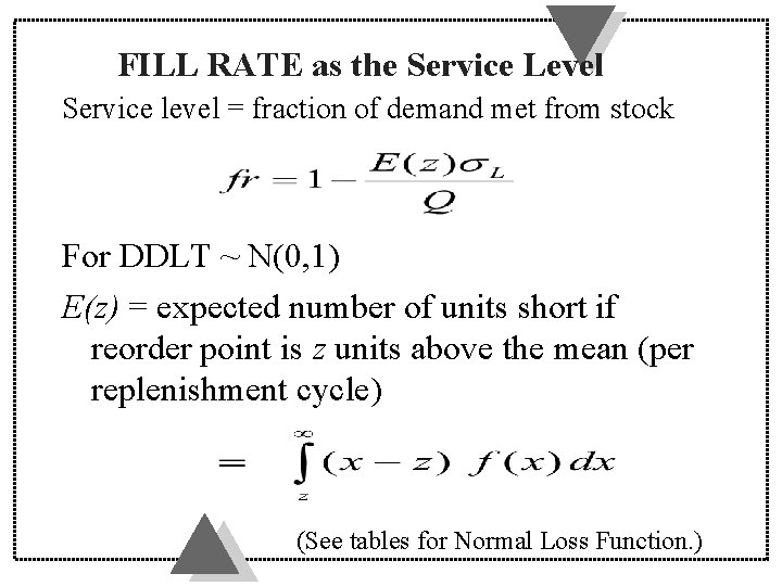
FILL RATE as the Service Level Service level = fraction of demand met from stock For DDLT ~ N(0, 1) E(z) = expected number of units short if reorder point is z units above the mean (per replenishment cycle) (See tables for Normal Loss Function. )

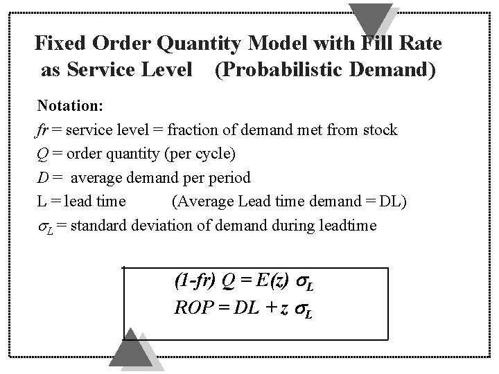
Fixed Order Quantity Model with Fill Rate as Service Level (Probabilistic Demand) Notation: fr = service level = fraction of demand met from stock Q = order quantity (per cycle) D = average demand period L = lead time (Average Lead time demand = DL) L = standard deviation of demand during leadtime (1 -fr) Q = E(z) L ROP = DL + z L

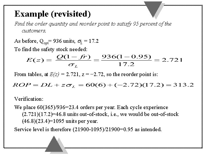
Example (revisited) Find the order quantity and reorder point to satisfy 95 percent of the customers. As before, Qopt= 936 units, L = 17. 2 To find the safety stock needed: From tables, at E(z) = 2. 721, z = − 2. 72, so the reorder point is: Verification: We place 60(365)/936=23. 4 orders per year. Each cycle experience (2. 721)(17. 2)=46. 8 units out-of-stock, i. e. , we would be out-of-stock (46. 8)(23. 4)=1095 units per year. Service level is therefore (21900 -1095)/21900=0. 95 as intended.

Factors Affecting Fill Rate u. Safety inventory: Fill rate increases if safety inventory is increased. This also increases the cycle service level. u. Lot size: Fill rate increases on increasing the lot size even though cycle service level does not change. Copyright © 2010 Pearson Education, Inc. Publishing as Prentice Hall. 11 -33

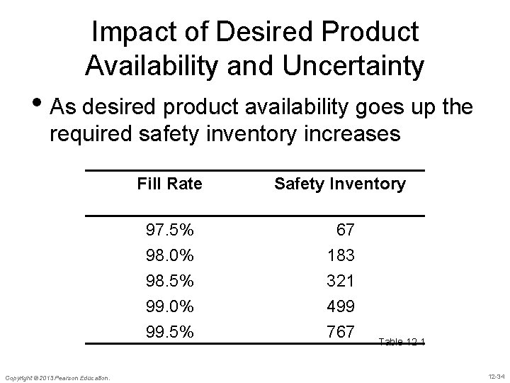
Impact of Desired Product Availability and Uncertainty • As desired product availability goes up the required safety inventory increases Copyright © 2013 Pearson Education. Fill Rate Safety Inventory 97. 5% 98. 0% 98. 5% 99. 0% 99. 5% 67 183 321 499 767 Table 12 -1 12 -34

Impact of Desired Product Availability and Uncertainty on Safety Inventory u. Desired product availability (cycle service level or fill rate) increases, required safety inventory increases u. Demand uncertainty ( L) increases, required safety inventory increases u. Managerial levers to reduce safety inventory without reducing product availability – reduce supplier lead time, L (better relationships with suppliers) – reduce uncertainty in demand, L (better forecasts, better information collection and use) Copyright © 2010 Pearson Education, Inc. Publishing as Prentice Hall. 11 -35

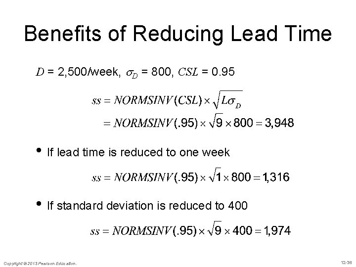
Benefits of Reducing Lead Time D = 2, 500/week, D = 800, CSL = 0. 95 • If lead time is reduced to one week • If standard deviation is reduced to 400 Copyright © 2013 Pearson Education. 12 -36

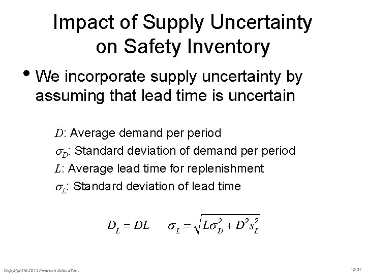
Impact of Supply Uncertainty on Safety Inventory • We incorporate supply uncertainty by assuming that lead time is uncertain D: Average demand period D: Standard deviation of demand period L: Average lead time for replenishment L: Standard deviation of lead time Copyright © 2013 Pearson Education. 12 -37

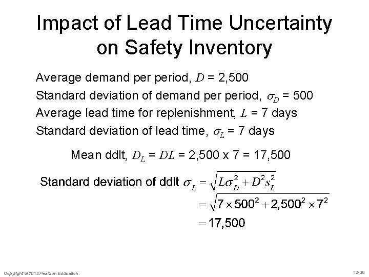
Impact of Lead Time Uncertainty on Safety Inventory Average demand period, D = 2, 500 Standard deviation of demand period, D = 500 Average lead time for replenishment, L = 7 days Standard deviation of lead time, L = 7 days Mean ddlt, DL = 2, 500 x 7 = 17, 500 Copyright © 2013 Pearson Education. 12 -38

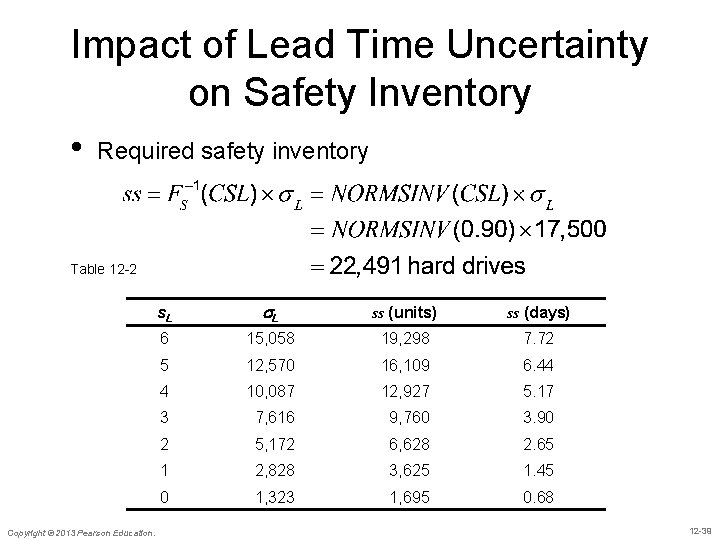
Impact of Lead Time Uncertainty on Safety Inventory • Required safety inventory Table 12 -2 Copyright © 2013 Pearson Education. s. L L ss (units) ss (days) 6 15, 058 19, 298 7. 72 5 12, 570 16, 109 6. 44 4 10, 087 12, 927 5. 17 3 7, 616 9, 760 3. 90 2 5, 172 6, 628 2. 65 1 2, 828 3, 625 1. 45 0 1, 323 1, 695 0. 68 12 -39

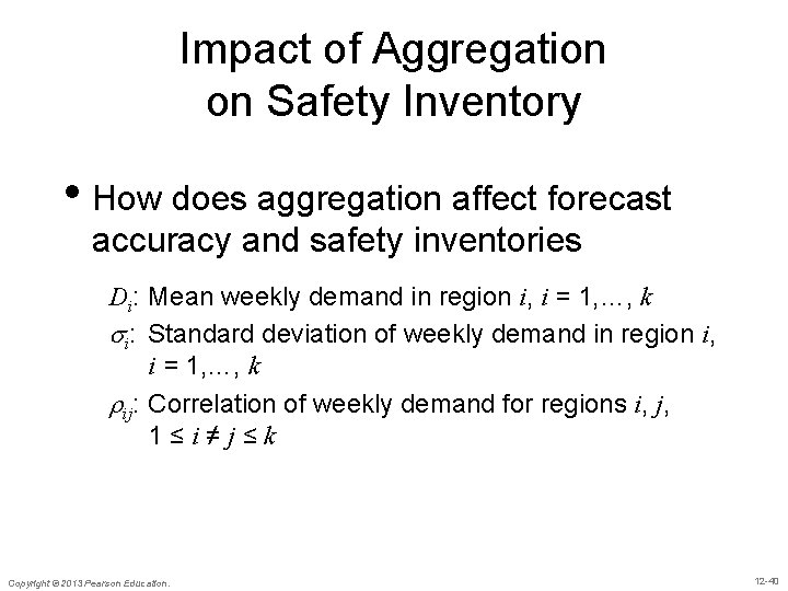
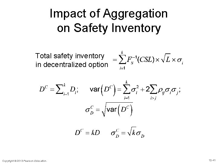
Impact of Aggregation on Safety Inventory • How does aggregation affect forecast accuracy and safety inventories Di: Mean weekly demand in region i, i = 1, …, k i: Standard deviation of weekly demand in region i, i = 1, …, k rij: Correlation of weekly demand for regions i, j, 1≤i≠j≤k Copyright © 2013 Pearson Education. 12 -40

Impact of Aggregation on Safety Inventory Total safety inventory in decentralized option Copyright © 2013 Pearson Education. 12 -41

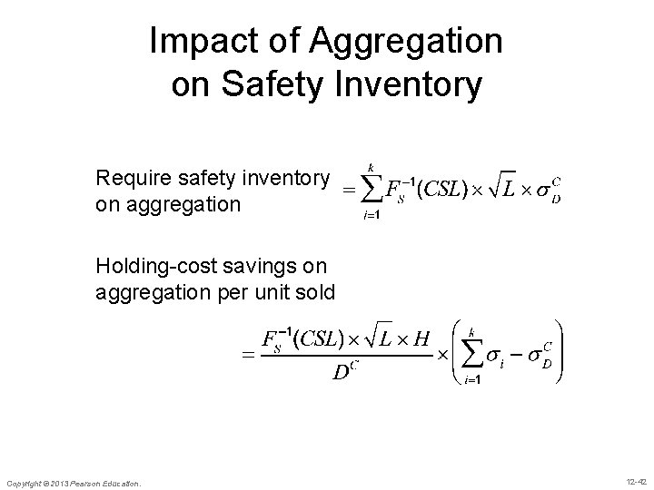
Impact of Aggregation on Safety Inventory Require safety inventory on aggregation Holding-cost savings on aggregation per unit sold Copyright © 2013 Pearson Education. 12 -42

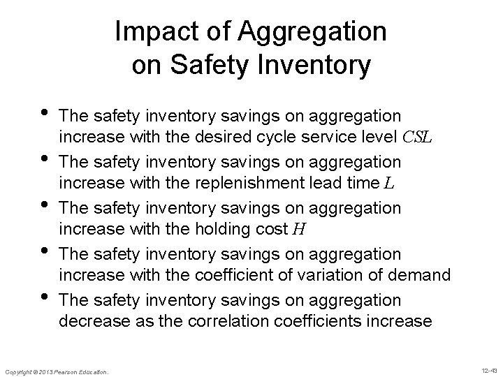
Impact of Aggregation on Safety Inventory • • • The safety inventory savings on aggregation increase with the desired cycle service level CSL The safety inventory savings on aggregation increase with the replenishment lead time L The safety inventory savings on aggregation increase with the holding cost H The safety inventory savings on aggregation increase with the coefficient of variation of demand The safety inventory savings on aggregation decrease as the correlation coefficients increase Copyright © 2013 Pearson Education. 12 -43

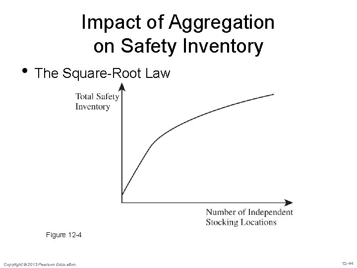
Impact of Aggregation on Safety Inventory • The Square-Root Law Figure 12 -4 Copyright © 2013 Pearson Education. 12 -44

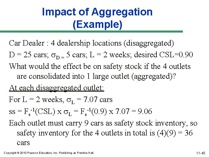
Impact of Aggregation (Example) Car Dealer : 4 dealership locations (disaggregated) D = 25 cars; D = 5 cars; L = 2 weeks; desired CSL=0. 90 What would the effect be on safety stock if the 4 outlets are consolidated into 1 large outlet (aggregated)? At each disaggregated outlet: For L = 2 weeks, L = 7. 07 cars ss = Fs-1(CSL) x L = Fs-1(0. 9) x 7. 07 = 9. 06 Each outlet must carry 9 cars as safety stock inventory, so safety inventory for the 4 outlets in total is (4)(9) = 36 cars Copyright © 2010 Pearson Education, Inc. Publishing as Prentice Hall. 11 -45

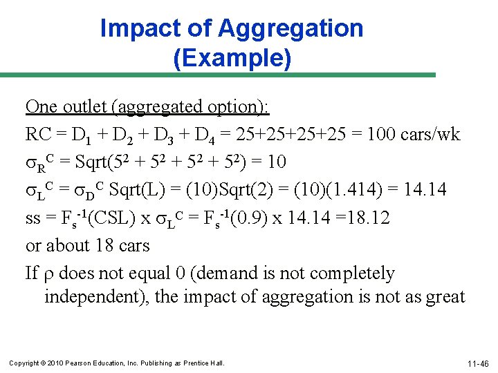
Impact of Aggregation (Example) One outlet (aggregated option): RC = D 1 + D 2 + D 3 + D 4 = 25+25+25+25 = 100 cars/wk RC = Sqrt(52 + 52) = 10 LC = DC Sqrt(L) = (10)Sqrt(2) = (10)(1. 414) = 14. 14 ss = Fs-1(CSL) x LC = Fs-1(0. 9) x 14. 14 =18. 12 or about 18 cars If r does not equal 0 (demand is not completely independent), the impact of aggregation is not as great Copyright © 2010 Pearson Education, Inc. Publishing as Prentice Hall. 11 -46

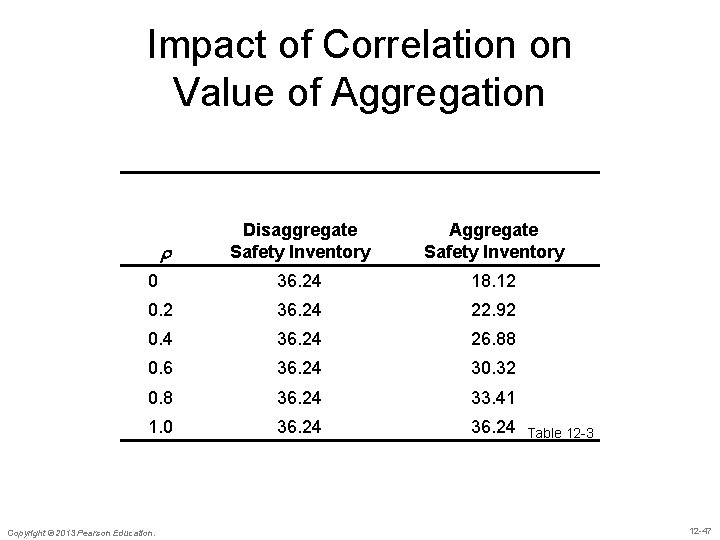
Impact of Correlation on Value of Aggregation Disaggregate Safety Inventory Aggregate Safety Inventory 0 36. 24 18. 12 0. 2 36. 24 22. 92 0. 4 36. 24 26. 88 0. 6 36. 24 30. 32 0. 8 36. 24 33. 41 1. 0 36. 24 r Copyright © 2013 Pearson Education. Table 12 -3 12 -47

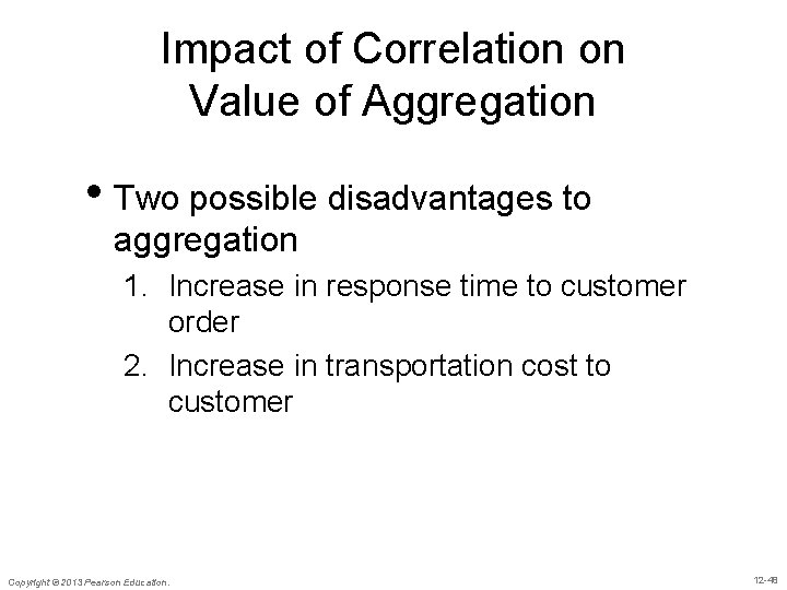
Impact of Correlation on Value of Aggregation • Two possible disadvantages to aggregation 1. Increase in response time to customer order 2. Increase in transportation cost to customer Copyright © 2013 Pearson Education. 12 -48

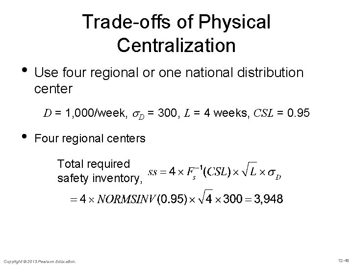
Trade-offs of Physical Centralization • Use four regional or one national distribution center D = 1, 000/week, D = 300, L = 4 weeks, CSL = 0. 95 • Four regional centers Total required safety inventory, Copyright © 2013 Pearson Education. 12 -49

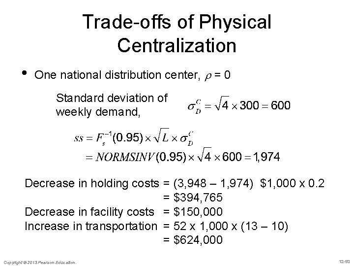
Trade-offs of Physical Centralization • One national distribution center, r = 0 Standard deviation of weekly demand, Decrease in holding costs = (3, 948 – 1, 974) $1, 000 x 0. 2 = $394, 765 Decrease in facility costs = $150, 000 Increase in transportation = 52 x 1, 000 x (13 – 10) = $624, 000 Copyright © 2013 Pearson Education. 12 -50

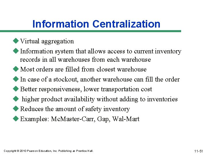
Information Centralization u Virtual aggregation u Information system that allows access to current inventory records in all warehouses from each warehouse u Most orders are filled from closest warehouse u In case of a stockout, another warehouse can fill the order u Better responsiveness, lower transportation cost u higher product availability without adding to inventories u Reduces the amount of safety inventory u Examples: Mc. Master-Carr, Gap, Wal-Mart Copyright © 2010 Pearson Education, Inc. Publishing as Prentice Hall. 11 -51

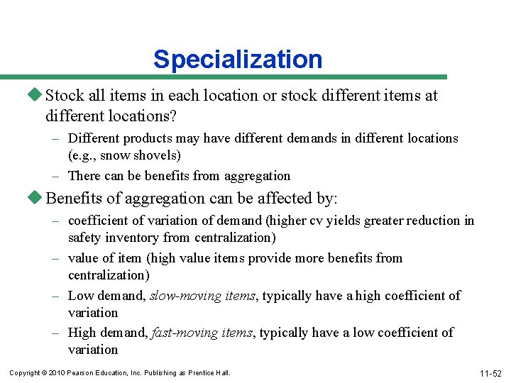
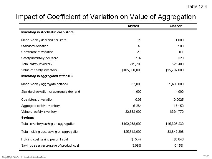
Specialization u Stock all items in each location or stock different items at different locations? – Different products may have different demands in different locations (e. g. , snow shovels) – There can be benefits from aggregation u Benefits of aggregation can be affected by: – coefficient of variation of demand (higher cv yields greater reduction in safety inventory from centralization) – value of item (high value items provide more benefits from centralization) – Low demand, slow-moving items, typically have a high coefficient of variation – High demand, fast-moving items, typically have a low coefficient of variation Copyright © 2010 Pearson Education, Inc. Publishing as Prentice Hall. 11 -52

Table 12 -4 Impact of Coefficient of Variation on Value of Aggregation Motors Cleaner Inventory is stocked in each store Mean weekly demand per store 20 1, 000 Standard deviation 40 100 Coefficient of variation 2. 0 0. 1 Safety inventory per store 132 329 211, 200 526, 400 $105, 600, 000 $15, 792, 000 32, 000 1, 600 4, 000 0. 05 0. 0025 5, 264 13, 159 $2, 632, 000 $394, 770 $102, 968, 000 $15, 397, 230 $25, 742, 000 $3, 849, 308 Holding cost saving per unit sold $15. 47 $0. 046 Savings as a percentage of product cost 3. 09% 0. 15% Total safety inventory Value of safety inventory Inventory is aggregated at the DC Mean weekly aggregate demand Standard deviation of aggregate demand Coefficient of variation Aggregate safety inventory Value of safety inventory Savings Total inventory saving on aggregation Total holding cost saving on aggregation Copyright © 2013 Pearson Education. 12 -53

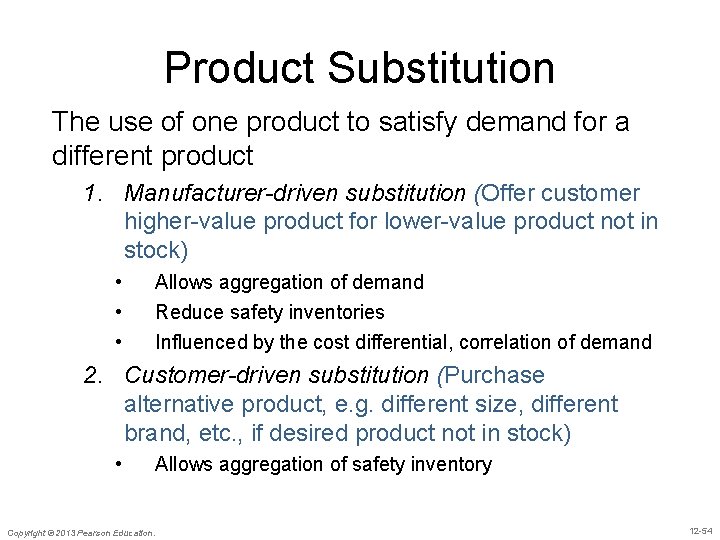
Product Substitution The use of one product to satisfy demand for a different product 1. Manufacturer-driven substitution (Offer customer higher-value product for lower-value product not in stock) • • • Allows aggregation of demand Reduce safety inventories Influenced by the cost differential, correlation of demand 2. Customer-driven substitution (Purchase alternative product, e. g. different size, different brand, etc. , if desired product not in stock) • Allows aggregation of safety inventory Copyright © 2013 Pearson Education. 12 -54

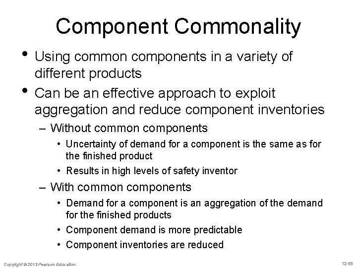
Component Commonality • Using common components in a variety of • different products Can be an effective approach to exploit aggregation and reduce component inventories – Without common components • Uncertainty of demand for a component is the same as for the finished product • Results in high levels of safety inventor – With common components • Demand for a component is an aggregation of the demand for the finished products • Component demand is more predictable • Component inventories are reduced Copyright © 2013 Pearson Education. 12 -55

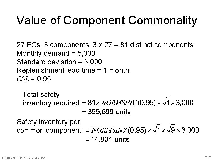
Value of Component Commonality 27 PCs, 3 components, 3 x 27 = 81 distinct components Monthly demand = 5, 000 Standard deviation = 3, 000 Replenishment lead time = 1 month CSL = 0. 95 Total safety inventory required Safety inventory per common component Copyright © 2013 Pearson Education. 12 -56

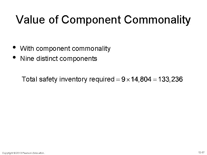
Value of Component Commonality • • With component commonality Nine distinct components Total safety inventory required Copyright © 2013 Pearson Education. 12 -57

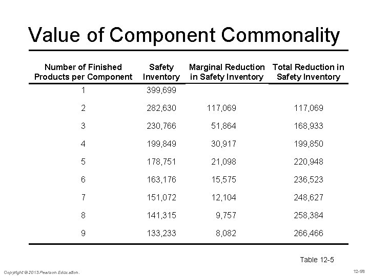
Value of Component Commonality Number of Finished Products per Component Safety Inventory Marginal Reduction Total Reduction in in Safety Inventory 1 399, 699 2 282, 630 117, 069 3 230, 766 51, 864 168, 933 4 199, 849 30, 917 199, 850 5 178, 751 21, 098 220, 948 6 163, 176 15, 575 236, 523 7 151, 072 12, 104 248, 627 8 141, 315 9, 757 258, 384 9 133, 233 8, 082 266, 466 Table 12 -5 Copyright © 2013 Pearson Education. 12 -58

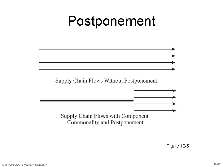
Postponement • Delay product differentiation or customization until closer to the time the product is sold – Have common components in the supply chain for most of the push phase – Move product differentiation as close to the pull phase of the supply chain as possible – Inventories in the supply chain are mostly aggregate e. g. Benetton Copyright © 2013 Pearson Education. 12 -59

Postponement Figure 12 -5 Copyright © 2013 Pearson Education. 12 -60

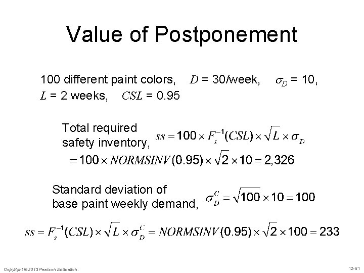
Value of Postponement 100 different paint colors, D = 30/week, L = 2 weeks, CSL = 0. 95 D = 10, Total required safety inventory, Standard deviation of base paint weekly demand, Copyright © 2013 Pearson Education. 12 -61

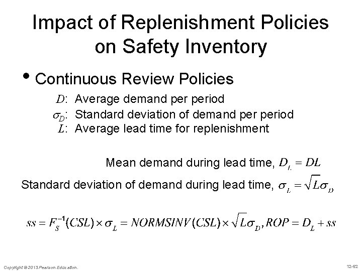
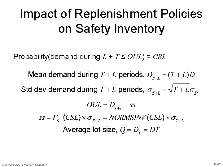
Impact of Replenishment Policies on Safety Inventory • Continuous Review Policies D: Average demand period D: Standard deviation of demand period L: Average lead time for replenishment Mean demand during lead time, Standard deviation of demand during lead time, Copyright © 2013 Pearson Education. 12 -62

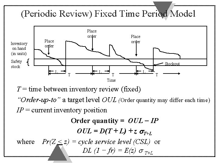
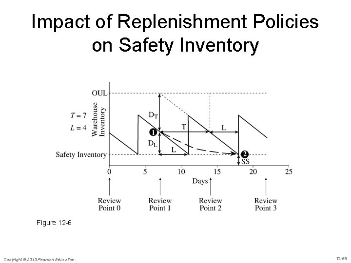
(Periodic Review) Fixed Time Period Model Place order Inventory on hand (in units) Place order Safety stock Stockout L T Time L T T = time between inventory review (fixed) “Order-up-to” a target level OUL (Order quantity may differ each time) IP = current inventory position Order quantity = OUL IP OUL = D(T + L) + z T+L where Pr(Z < z) = cycle service level (CSL) or DL (1 − fr) = E(z) T+L

Impact of Replenishment Policies on Safety Inventory • Periodic Review Policies – Lot size determined by prespecified order-upto level (OUL) D: D : L: T: CSL: Copyright © 2013 Pearson Education. Average demand period Standard deviation of demand period Average lead time for replenishment Review interval Desired cycle service level 12 -64

Impact of Replenishment Policies on Safety Inventory Probability(demand during L + T ≤ OUL) = CSL Copyright © 2013 Pearson Education. 12 -65

Impact of Replenishment Policies on Safety Inventory Figure 12 -6 Copyright © 2013 Pearson Education. 12 -66

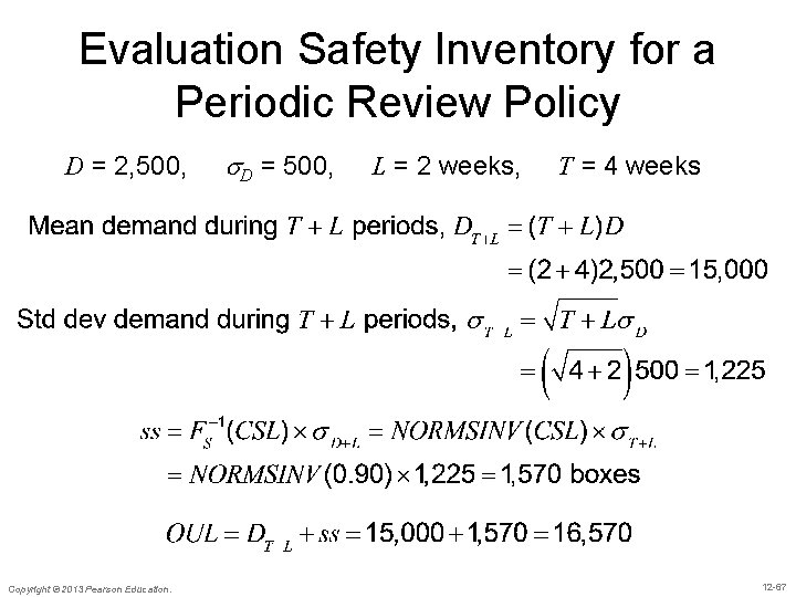
Evaluation Safety Inventory for a Periodic Review Policy D = 2, 500, Copyright © 2013 Pearson Education. D = 500, L = 2 weeks, T = 4 weeks 12 -67

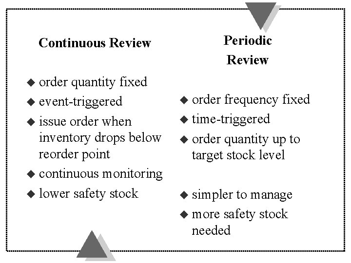
Periodic Review Continuous Review u order quantity fixed u event-triggered u issue order when inventory drops below reorder point u continuous monitoring u lower safety stock u order frequency fixed u time-triggered u order quantity up to target stock level u simpler to manage u more safety stock needed

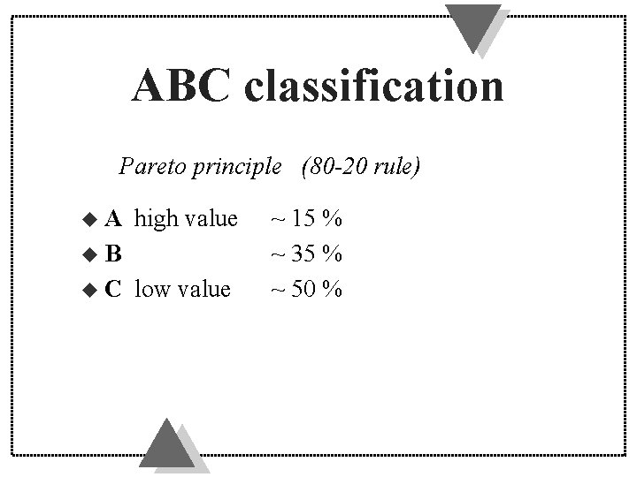
ABC classification Pareto principle (80 -20 rule) u. A high value u. B u. C low value ~ 15 % ~ 35 % ~ 50 %

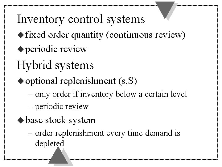
Inventory control systems u fixed order quantity (continuous review) u periodic review Hybrid systems u optional replenishment (s, S) – only order if inventory below a certain level – periodic review u base stock system – order replenishment every time demand is depleted

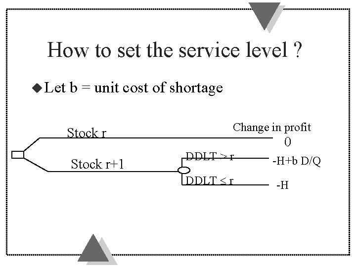
How to set the service level ? u Let b = unit cost of shortage Stock r+1 Change in profit 0 DDLT > r DDLT r -H+b D/Q -H

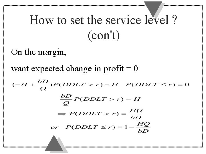
How to set the service level ? (con't) On the margin, want expected change in profit = 0

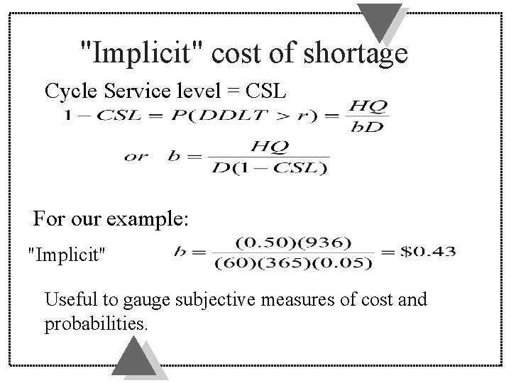
"Implicit" cost of shortage Cycle Service level = CSL For our example: "Implicit" Useful to gauge subjective measures of cost and probabilities.

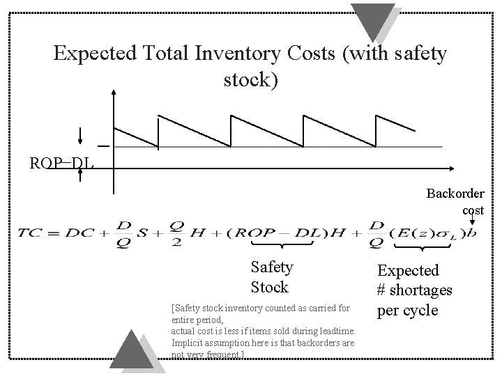
Expected Total Inventory Costs (with safety stock) ROP−DL Backorder cost Safety Stock [Safety stock inventory counted as carried for entire period, actual cost is less if items sold during leadtime. Implicit assumption here is that backorders are not very frequent. ] Expected # shortages per cycle

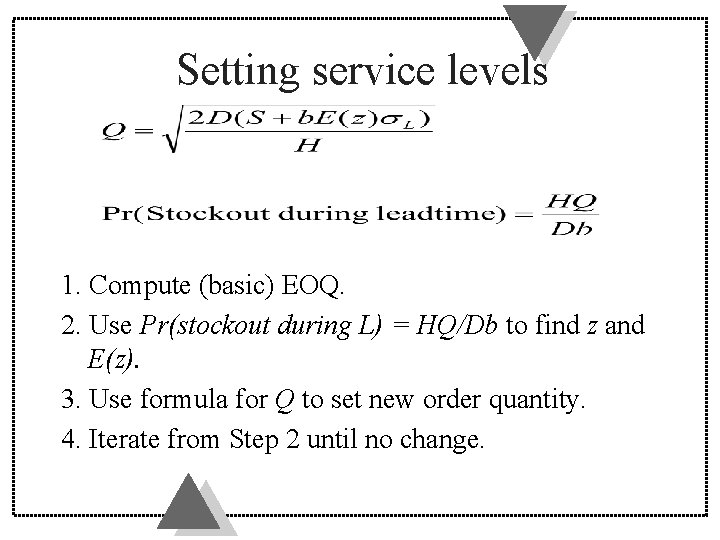
Setting service levels 1. Compute (basic) EOQ. 2. Use Pr(stockout during L) = HQ/Db to find z and E(z). 3. Use formula for Q to set new order quantity. 4. Iterate from Step 2 until no change.

Managing Safety Inventory in a Multi-echelon Supply Chain • In multiechelon supply chains stages often do • • • not know demand supply distributions Inventory between a stage and the final customer is called the echelon inventory Reorder points and order-up-to levels at any stage should be based on echelon inventory Decisions must be made about the level of safety inventory carried at different stages Copyright © 2013 Pearson Education. 12 -76

The Role of IT in Inventory Management • IT systems can help – Improve inventory visibility – Coordination in the supply chain – Track inventory (RFID) • Value tightly linked to the accuracy of the inventory information Copyright © 2013 Pearson Education. 12 -77

Estimating and Managing Safety Inventory in Practice 1. Account for the fact that supply chain demand is lumpy 2. Adjust inventory policies if demand is seasonal 3. Use simulation to test inventory policies 4. Start with a pilot 5. Monitor service levels 6. Focus on reducing safety inventories Copyright © 2013 Pearson Education. 12 -78

Summary of Learning Objectives 1. Understand the role of safety inventory in a supply chain 2. Identify factors that influence the required level of safety inventory 3. Describe different measures of product availability 4. Utilize managerial levers available to lower safety inventory and improve product availability Copyright © 2013 Pearson Education. 12 -79

All rights reserved. No part of this publication may be reproduced, stored in a retrieval system, or transmitted, in any form or by any means, electronic, mechanical, photocopying, recording, or otherwise, without the prior written permission of the publisher. Printed in the United States of America. Copyright © 2013 Pearson Education. 12 -80