11 Managing Economies of Scale in a Supply

11 Managing Economies of Scale in a Supply Chain: Cycle Inventory Power. Point presentation to accompany Chopra and Meindl Supply Chain Management, 5 e Global Edition Copyright © 2013 Pearson Education. 11 -1

Learning Objectives 1. Balance the appropriate costs to choose the optimal lot size and cycle inventory in a supply chain. 2. Understand the impact of quantity discounts on lot size and cycle inventory. 3. Devise appropriate discounting schemes for a supply chain. 4. Understand the impact of trade promotions on lot size and cycle inventory. 5. Identify managerial levers that reduce lot size and cycle inventory in a supply chain without increasing cost. Copyright © 2013 Pearson Education. 11 -2

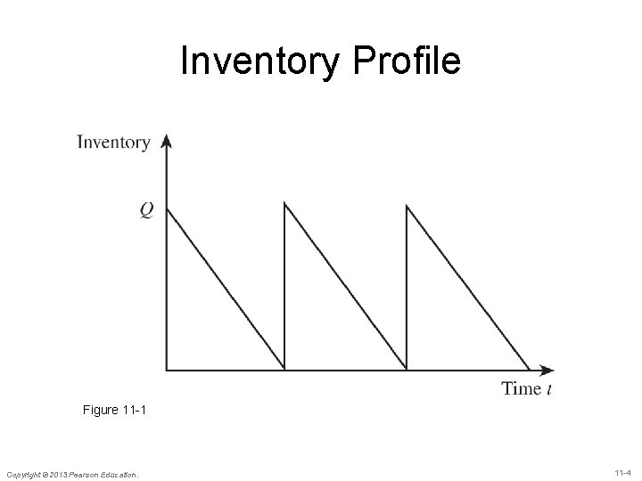
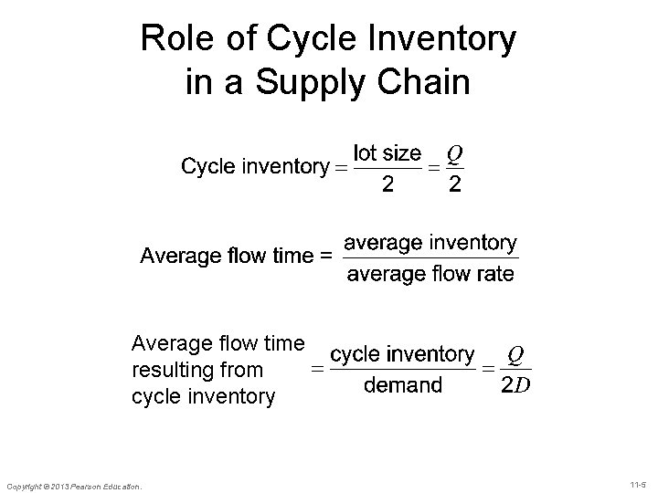
Role of Cycle Inventory in a Supply Chain • Lot or batch size is the quantity that a • stage of a supply chain either produces or purchases at a time Cycle inventory is the average inventory in a supply chain due to either production or purchases in lot sizes that are larger than those demanded by the customer Q: Quantity in a lot or batch size D: Demand per unit time Copyright © 2013 Pearson Education. 11 -3

Inventory Profile Figure 11 -1 Copyright © 2013 Pearson Education. 11 -4

Role of Cycle Inventory in a Supply Chain Average flow time resulting from cycle inventory Copyright © 2013 Pearson Education. 11 -5

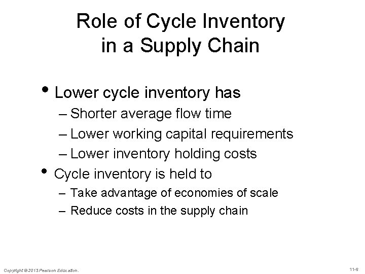
Role of Cycle Inventory in a Supply Chain • Lower cycle inventory has • – Shorter average flow time – Lower working capital requirements – Lower inventory holding costs Cycle inventory is held to – Take advantage of economies of scale – Reduce costs in the supply chain Copyright © 2013 Pearson Education. 11 -6

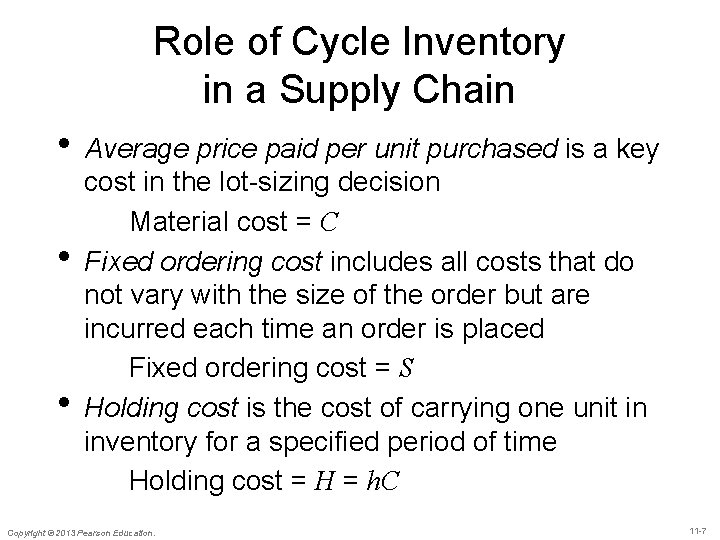
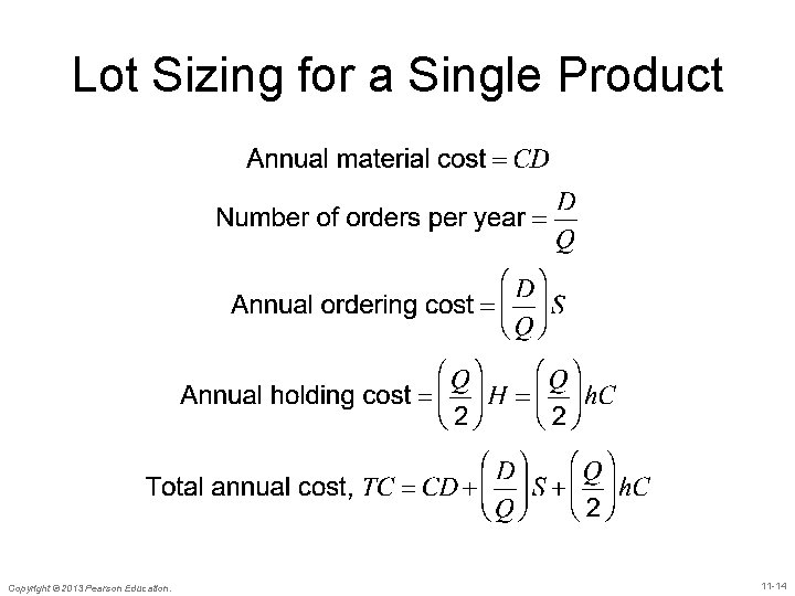
Role of Cycle Inventory in a Supply Chain • Average price paid per unit purchased is a key • • cost in the lot-sizing decision Material cost = C Fixed ordering cost includes all costs that do not vary with the size of the order but are incurred each time an order is placed Fixed ordering cost = S Holding cost is the cost of carrying one unit in inventory for a specified period of time Holding cost = H = h. C Copyright © 2013 Pearson Education. 11 -7

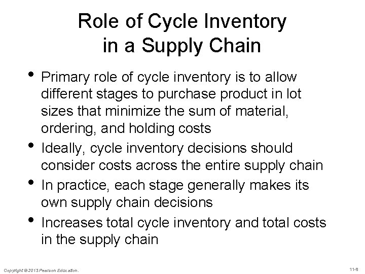
Role of Cycle Inventory in a Supply Chain • Primary role of cycle inventory is to allow • • • different stages to purchase product in lot sizes that minimize the sum of material, ordering, and holding costs Ideally, cycle inventory decisions should consider costs across the entire supply chain In practice, each stage generally makes its own supply chain decisions Increases total cycle inventory and total costs in the supply chain Copyright © 2013 Pearson Education. 11 -8

Role of Cycle Inventory in a Supply Chain • Economies of scale exploited in three typical situations 1. A fixed cost is incurred each time an order is placed or produced 2. The supplier offers price discounts based on the quantity purchased per lot 3. The supplier offers short-term price discounts or holds trade promotions Copyright © 2013 Pearson Education. 11 -9

Estimating Cycle Inventory Related Costs in Practice • Inventory Holding Cost – Obsolescence cost – Handling cost – Occupancy cost – Miscellaneous costs • Theft, security, damage, tax, insurance Copyright © 2013 Pearson Education. 11 -10

Estimating Cycle Inventory Related Costs in Practice • Ordering Cost – Buyer time – Transportation costs – Receiving costs – Other costs Copyright © 2013 Pearson Education. 11 -11

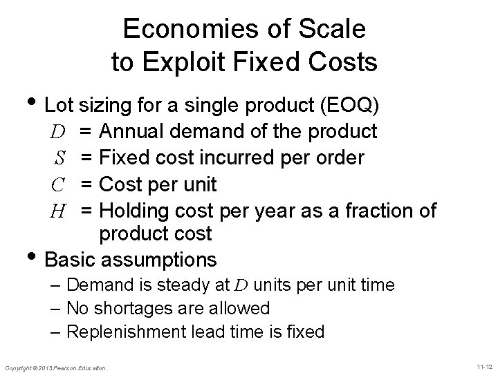
Economies of Scale to Exploit Fixed Costs • Lot sizing for a single product (EOQ) Annual demand of the product Fixed cost incurred per order Cost per unit Holding cost per year as a fraction of product cost Basic assumptions D S C H • = = – Demand is steady at D units per unit time – No shortages are allowed – Replenishment lead time is fixed Copyright © 2013 Pearson Education. 11 -12

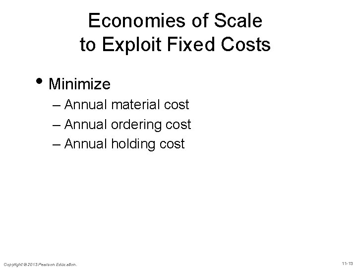
Economies of Scale to Exploit Fixed Costs • Minimize – Annual material cost – Annual ordering cost – Annual holding cost Copyright © 2013 Pearson Education. 11 -13

Lot Sizing for a Single Product Copyright © 2013 Pearson Education. 11 -14

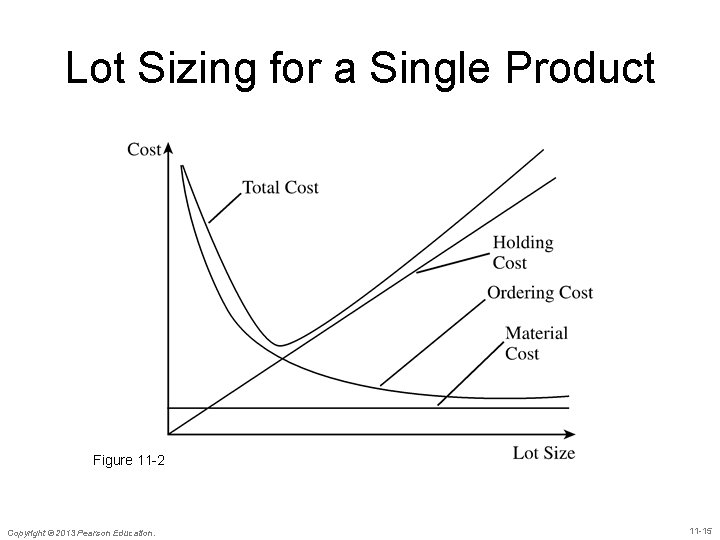
Lot Sizing for a Single Product Figure 11 -2 Copyright © 2013 Pearson Education. 11 -15

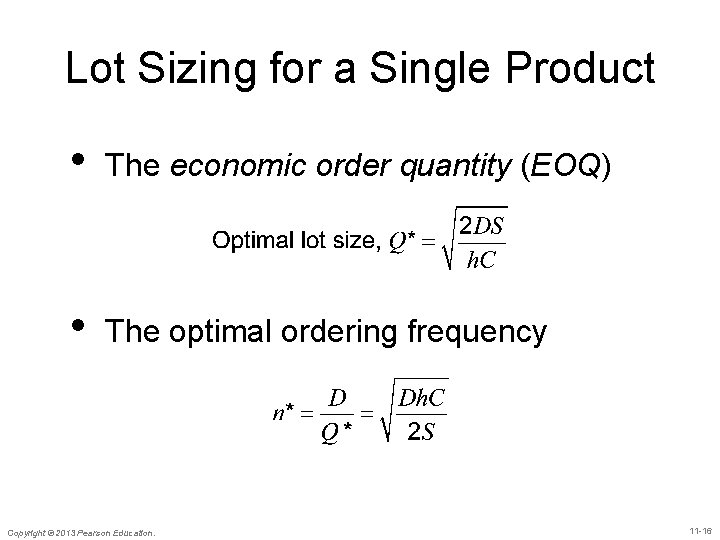
Lot Sizing for a Single Product • The economic order quantity (EOQ) • The optimal ordering frequency Copyright © 2013 Pearson Education. 11 -16

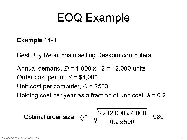
EOQ Example 11 -1 Best Buy Retail chain selling Deskpro computers Annual demand, D = 1, 000 x 12 = 12, 000 units Order cost per lot, S = $4, 000 Unit cost per computer, C = $500 Holding cost per year as a fraction of unit cost, h = 0. 2 Copyright © 2013 Pearson Education. 11 -17

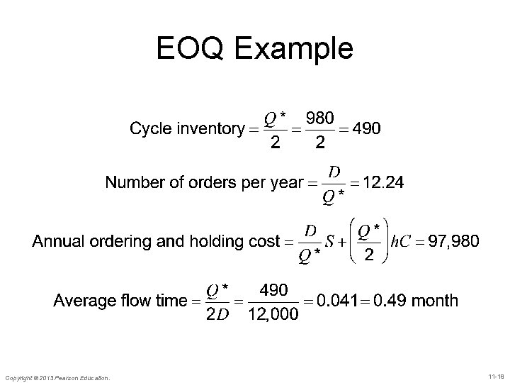
EOQ Example Copyright © 2013 Pearson Education. 11 -18

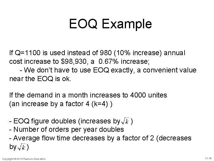
EOQ Example If Q=1100 is used instead of 980 (10% increase) annual cost increase to $98, 930, a 0. 67% increase; - We don’t have to use EOQ exactly, a convenient value near the EOQ is ok. If the demand in a month increases to 4000 unites (an increase by a factor 4 (k=4) ) - EOQ figure doubles (increases by ) - Number of orders per year doubles - Average flow time decreases by a factor of 2 (decreases by ) Copyright © 2013 Pearson Education. 11 -19

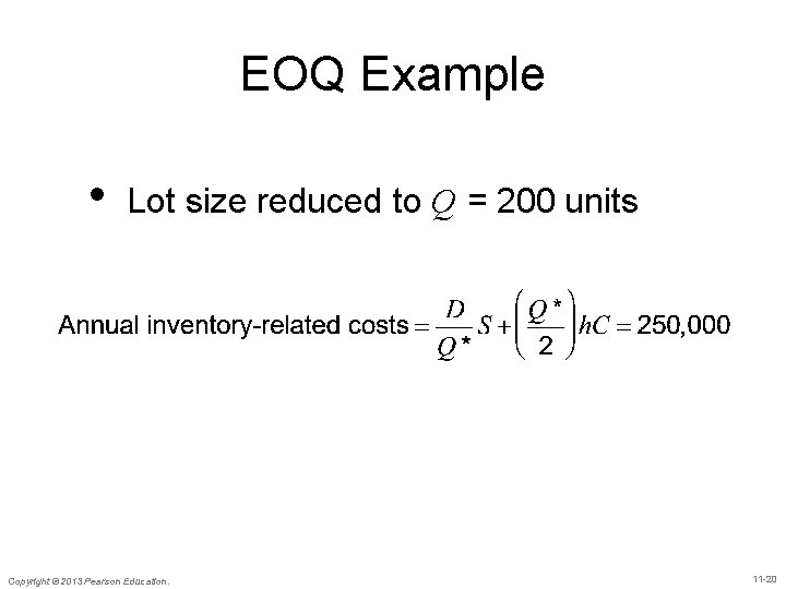
EOQ Example • Lot size reduced to Q = 200 units Copyright © 2013 Pearson Education. 11 -20

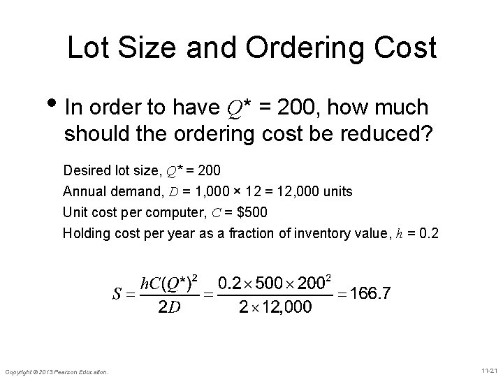
Lot Size and Ordering Cost • In order to have Q* = 200, how much should the ordering cost be reduced? Desired lot size, Q* = 200 Annual demand, D = 1, 000 × 12 = 12, 000 units Unit cost per computer, C = $500 Holding cost per year as a fraction of inventory value, h = 0. 2 Copyright © 2013 Pearson Education. 11 -21

Aggregating Multiple Products in a Single Order • Single delivery from multiple suppliers or • single truck delivering to multiple retailers Savings in transportation costs – Reduces fixed cost for each product – Lot size for each product can be reduced – Cycle inventory is reduced • Receiving and loading costs can be reduced using ASP(advance shipping notice), RFID, badcode Copyright © 2013 Pearson Education. 11 -22

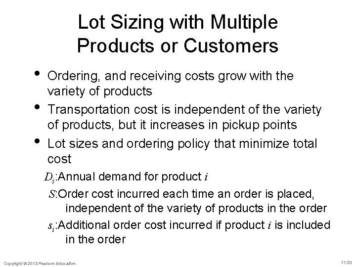
Lot Sizing with Multiple Products or Customers • • • Ordering, and receiving costs grow with the variety of products Transportation cost is independent of the variety of products, but it increases in pickup points Lot sizes and ordering policy that minimize total cost Di: Annual demand for product i S: Order cost incurred each time an order is placed, independent of the variety of products in the order si: Additional order cost incurred if product i is included in the order Copyright © 2013 Pearson Education. 11 -23

Lot Sizing with Multiple Products or Customers • Three approaches 1. Each product manager orders his or her model independently 2. The product managers jointly order every product in each lot 3. Product managers order jointly but not every order contains every product; that is, each lot contains a selected subset of the products Copyright © 2013 Pearson Education. 11 -24

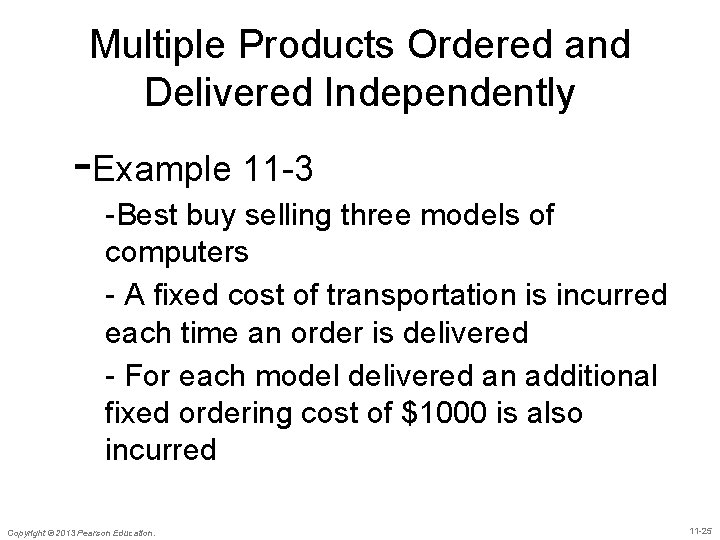
Multiple Products Ordered and Delivered Independently -Example 11 -3 -Best buy selling three models of computers - A fixed cost of transportation is incurred each time an order is delivered - For each model delivered an additional fixed ordering cost of $1000 is also incurred Copyright © 2013 Pearson Education. 11 -25

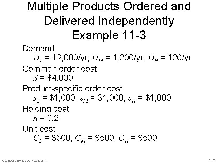
Multiple Products Ordered and Delivered Independently Example 11 -3 Demand DL = 12, 000/yr, DM = 1, 200/yr, DH = 120/yr Common order cost S = $4, 000 Product-specific order cost s. L = $1, 000, s. M = $1, 000, s. H = $1, 000 Holding cost h = 0. 2 Unit cost CL = $500, CM = $500, CH = $500 Copyright © 2013 Pearson Education. 11 -26

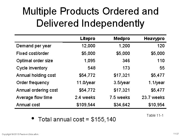
Multiple Products Ordered and Delivered Independently Litepro Medpro Heavypro Demand per year 12, 000 1, 200 120 Fixed cost/order $5, 000 1, 095 346 110 548 173 55 $54, 772 $17, 321 $5, 477 11. 0/year 3. 5/year 1. 1/year $54, 772 $17, 321 $5, 477 2. 4 weeks 7. 5 weeks 23. 7 weeks $109, 544 $34, 642 $10, 954 Optimal order size Cycle inventory Annual holding cost Order frequency Annual ordering cost Average flow time Annual cost • Total annual cost = $155, 140 Copyright © 2013 Pearson Education. Table 11 -1 11 -27

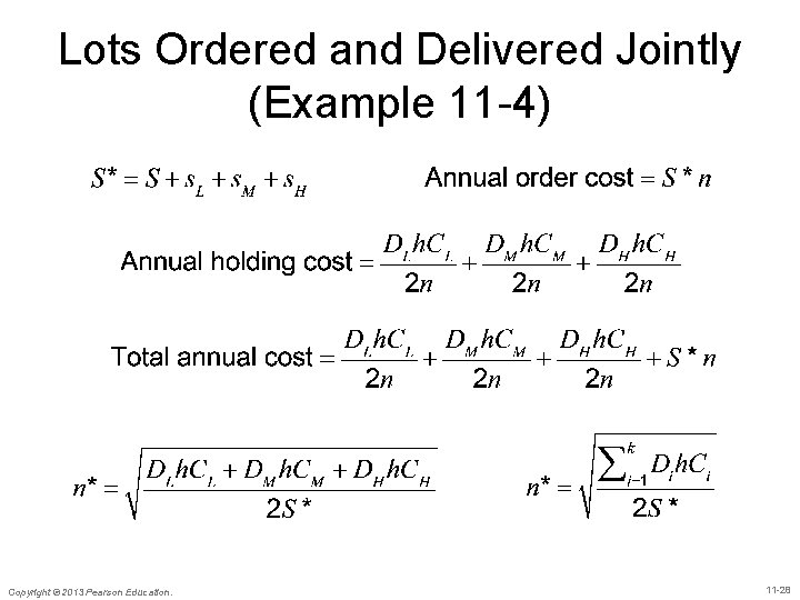
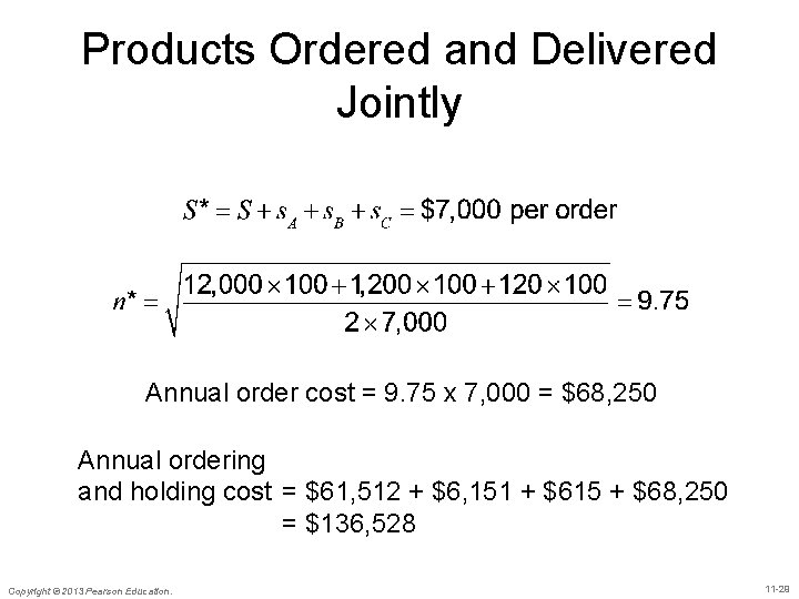
Lots Ordered and Delivered Jointly (Example 11 -4) Copyright © 2013 Pearson Education. 11 -28

Products Ordered and Delivered Jointly Annual order cost = 9. 75 x 7, 000 = $68, 250 Annual ordering and holding cost = $61, 512 + $6, 151 + $615 + $68, 250 = $136, 528 Copyright © 2013 Pearson Education. 11 -29

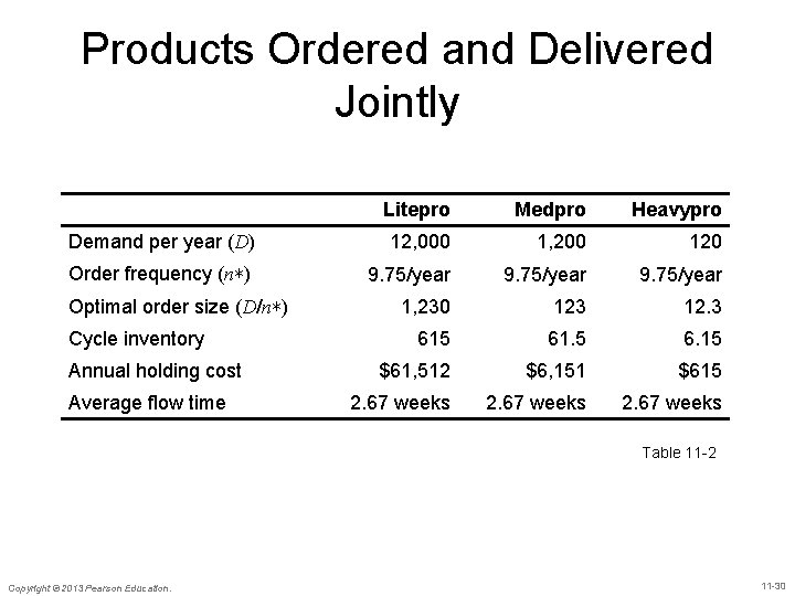
Products Ordered and Delivered Jointly Litepro Medpro Heavypro Demand per year (D) 12, 000 1, 200 120 Order frequency (n∗) 9. 75/year 1, 230 123 12. 3 615 61. 5 6. 15 $61, 512 $6, 151 $615 2. 67 weeks Optimal order size (D/n∗) Cycle inventory Annual holding cost Average flow time Table 11 -2 Copyright © 2013 Pearson Education. 11 -30

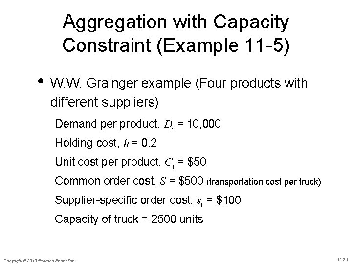
Aggregation with Capacity Constraint (Example 11 -5) • W. W. Grainger example (Four products with different suppliers) Demand per product, Di = 10, 000 Holding cost, h = 0. 2 Unit cost per product, Ci = $50 Common order cost, S = $500 (transportation cost per truck) Supplier-specific order cost, si = $100 Capacity of truck = 2500 units Copyright © 2013 Pearson Education. 11 -31

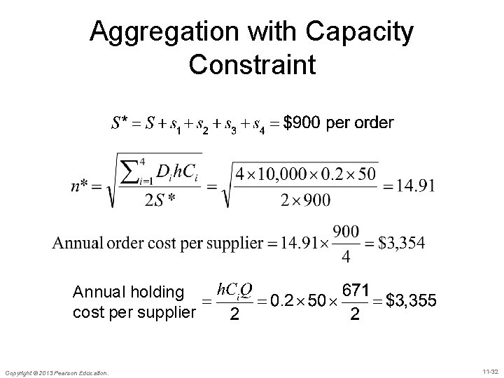
Aggregation with Capacity Constraint Annual holding cost per supplier Copyright © 2013 Pearson Education. 11 -32

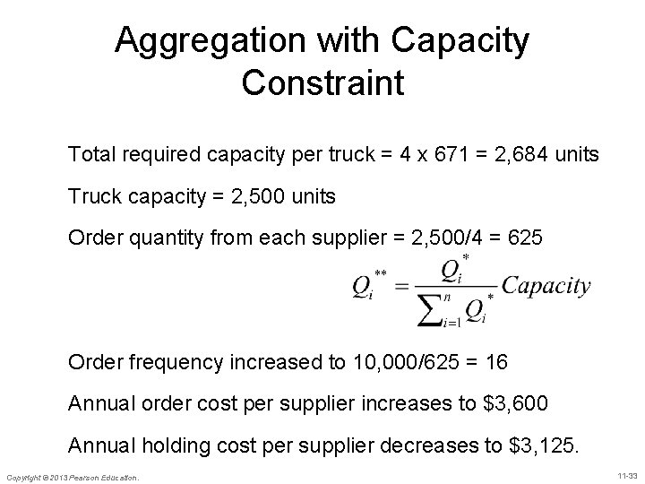
Aggregation with Capacity Constraint Total required capacity per truck = 4 x 671 = 2, 684 units Truck capacity = 2, 500 units Order quantity from each supplier = 2, 500/4 = 625 Order frequency increased to 10, 000/625 = 16 Annual order cost per supplier increases to $3, 600 Annual holding cost per supplier decreases to $3, 125. Copyright © 2013 Pearson Education. 11 -33

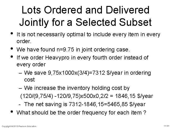
Lots Ordered and Delivered Jointly for a Selected Subset • • It is not necessarily optimal to include every item in every order. We have found n=9. 75 in joint ordering case. If we order Heavypro in every fourth order instead of every order – We save 9, 75 x 1000 x(3/4)=7312 $/year in ordering cost – We increase the inventory holding cost by (120/(9, 75/4) -120/9, 75)x 500 x 0, 2/2 = 1846, 15 $/year - The net saving is 7312 -1846, 15=5465, 85 $/year What should be the order frequency for each item ? Copyright © 2013 Pearson Education. 11 -34

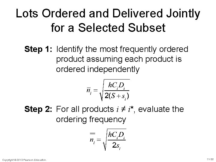
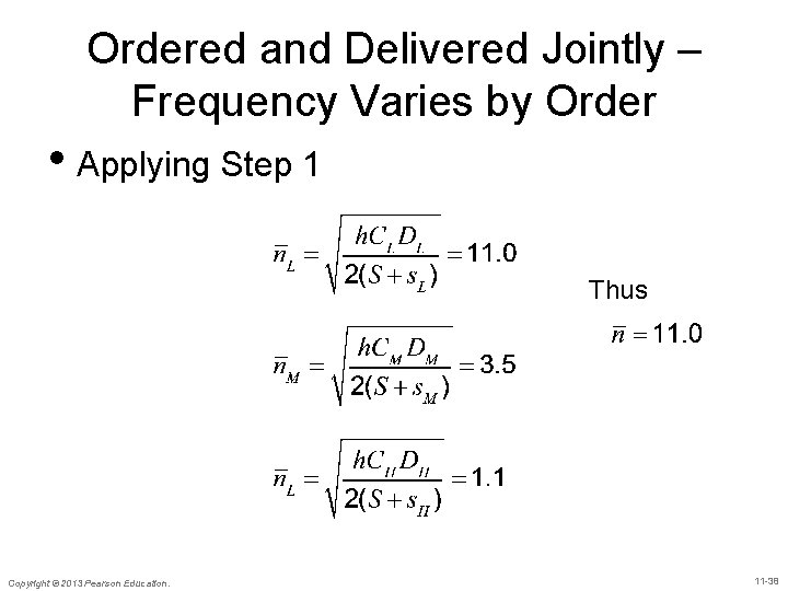
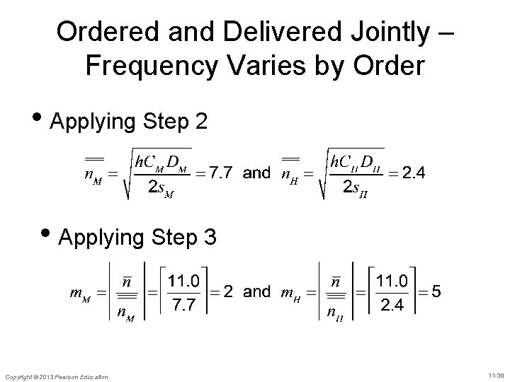
Lots Ordered and Delivered Jointly for a Selected Subset Step 1: Identify the most frequently ordered product assuming each product is ordered independently Step 2: For all products i ≠ i*, evaluate the ordering frequency Copyright © 2013 Pearson Education. 11 -35

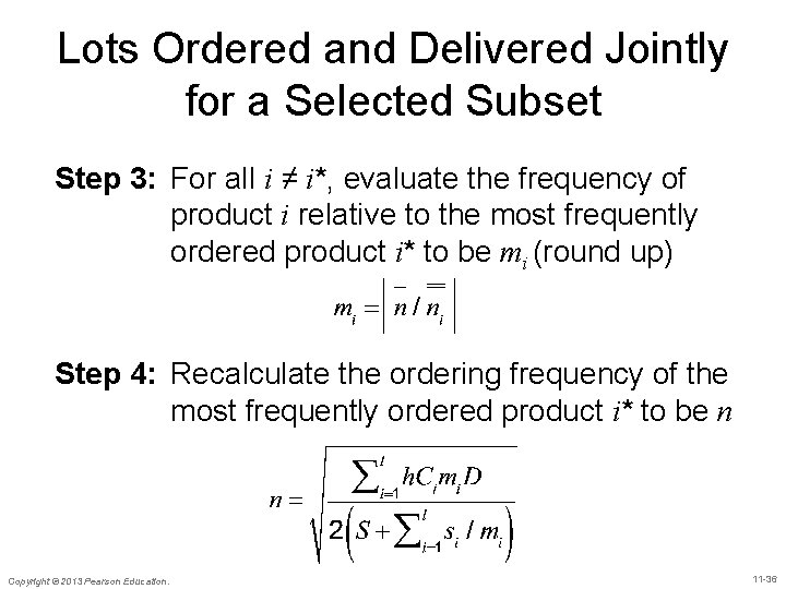
Lots Ordered and Delivered Jointly for a Selected Subset Step 3: For all i ≠ i*, evaluate the frequency of product i relative to the most frequently ordered product i* to be mi (round up) Step 4: Recalculate the ordering frequency of the most frequently ordered product i* to be n Copyright © 2013 Pearson Education. 11 -36

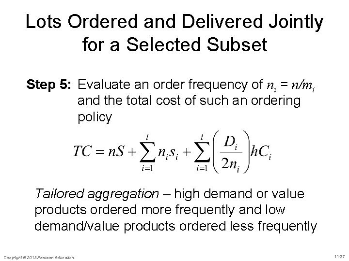
Lots Ordered and Delivered Jointly for a Selected Subset Step 5: Evaluate an order frequency of ni = n/mi and the total cost of such an ordering policy Tailored aggregation – high demand or value products ordered more frequently and low demand/value products ordered less frequently Copyright © 2013 Pearson Education. 11 -37

Ordered and Delivered Jointly – Frequency Varies by Order • Applying Step 1 Thus Copyright © 2013 Pearson Education. 11 -38

Ordered and Delivered Jointly – Frequency Varies by Order • Applying Step 2 • Applying Step 3 Copyright © 2013 Pearson Education. 11 -39

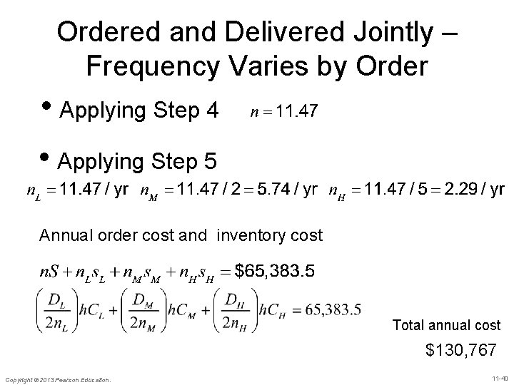
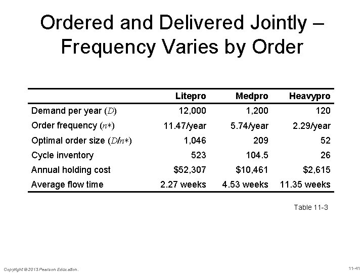
Ordered and Delivered Jointly – Frequency Varies by Order • Applying Step 4 • Applying Step 5 Annual order cost and inventory cost Total annual cost $130, 767 Copyright © 2013 Pearson Education. 11 -40

Ordered and Delivered Jointly – Frequency Varies by Order Litepro Medpro Heavypro Demand per year (D) 12, 000 1, 200 120 Order frequency (n∗) 11. 47/year 5. 74/year 2. 29/year 1, 046 209 52 523 104. 5 26 $52, 307 $10, 461 $2, 615 2. 27 weeks 4. 53 weeks 11. 35 weeks Optimal order size (D/n∗) Cycle inventory Annual holding cost Average flow time Table 11 -3 Copyright © 2013 Pearson Education. 11 -41

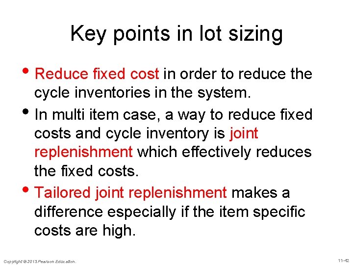
Key points in lot sizing • Reduce fixed cost in order to reduce the • • cycle inventories in the system. In multi item case, a way to reduce fixed costs and cycle inventory is joint replenishment which effectively reduces the fixed costs. Tailored joint replenishment makes a difference especially if the item specific costs are high. Copyright © 2013 Pearson Education. 11 -42

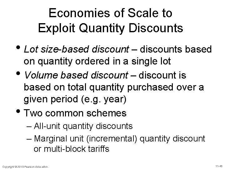
Economies of Scale to Exploit Quantity Discounts • Lot size-based discount – discounts based • • on quantity ordered in a single lot Volume based discount – discount is based on total quantity purchased over a given period (e. g. year) Two common schemes – All-unit quantity discounts – Marginal unit (incremental) quantity discount or multi-block tariffs Copyright © 2013 Pearson Education. 11 -43

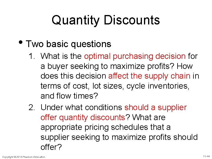
Quantity Discounts • Two basic questions 1. What is the optimal purchasing decision for a buyer seeking to maximize profits? How does this decision affect the supply chain in terms of cost, lot sizes, cycle inventories, and flow times? 2. Under what conditions should a supplier offer quantity discounts? What are appropriate pricing schedules that a supplier seeking to maximize profits should offer? Copyright © 2013 Pearson Education. 11 -44

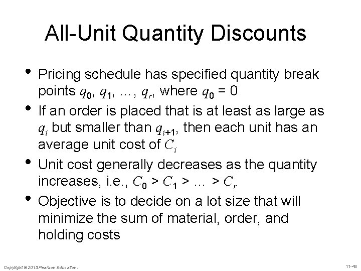
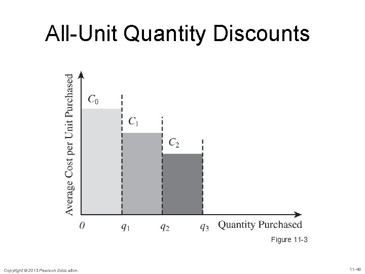
All-Unit Quantity Discounts • Pricing schedule has specified quantity break • • • points q 0, q 1, …, qr, where q 0 = 0 If an order is placed that is at least as large as qi but smaller than qi+1, then each unit has an average unit cost of Ci Unit cost generally decreases as the quantity increases, i. e. , C 0 > C 1 > … > Cr Objective is to decide on a lot size that will minimize the sum of material, order, and holding costs Copyright © 2013 Pearson Education. 11 -45

All-Unit Quantity Discounts Figure 11 -3 Copyright © 2013 Pearson Education. 11 -46

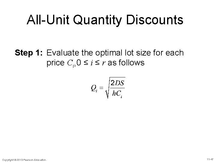
All-Unit Quantity Discounts Step 1: Evaluate the optimal lot size for each price Ci, 0 ≤ i ≤ r as follows Copyright © 2013 Pearson Education. 11 -47

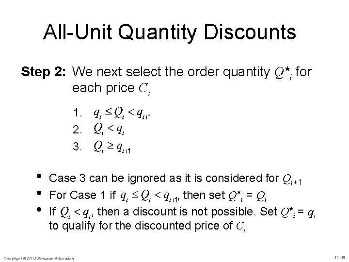
All-Unit Quantity Discounts Step 2: We next select the order quantity Q*i for each price Ci 1. 2. 3. • • • Case 3 can be ignored as it is considered for Qi+1 For Case 1 if , then set Q*i = Qi If , then a discount is not possible. Set Q*i = qi to qualify for the discounted price of Ci Copyright © 2013 Pearson Education. 11 -48

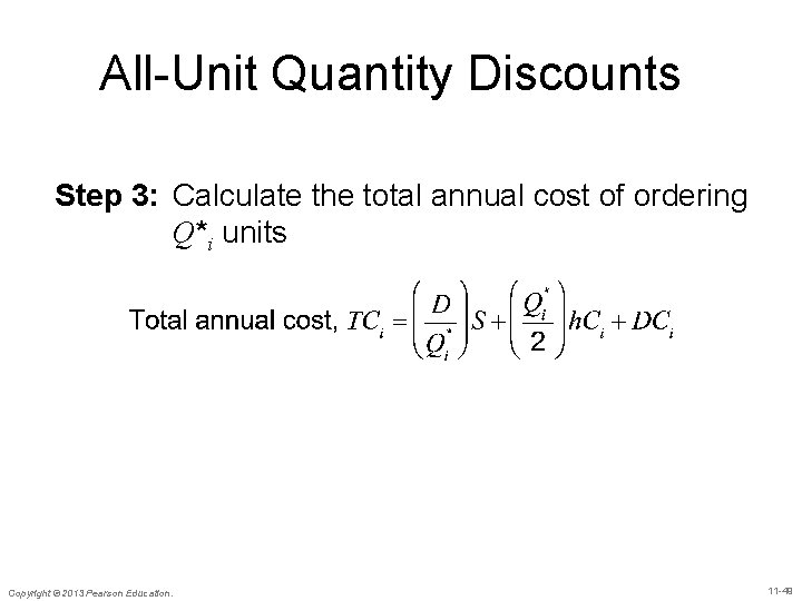
All-Unit Quantity Discounts Step 3: Calculate the total annual cost of ordering Q*i units Copyright © 2013 Pearson Education. 11 -49

All-Unit Quantity Discounts Step 4: Select Q*i with the lowest total cost TCi Copyright © 2013 Pearson Education. 11 -50

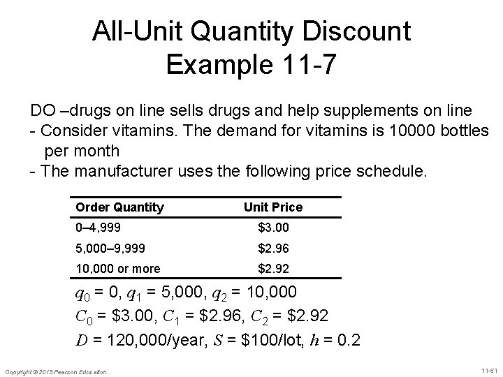
All-Unit Quantity Discount Example 11 -7 DO –drugs on line sells drugs and help supplements on line - Consider vitamins. The demand for vitamins is 10000 bottles per month - The manufacturer uses the following price schedule. Order Quantity Unit Price 0– 4, 999 $3. 00 5, 000– 9, 999 $2. 96 10, 000 or more $2. 92 q 0 = 0, q 1 = 5, 000, q 2 = 10, 000 C 0 = $3. 00, C 1 = $2. 96, C 2 = $2. 92 D = 120, 000/year, S = $100/lot, h = 0. 2 Copyright © 2013 Pearson Education. 11 -51

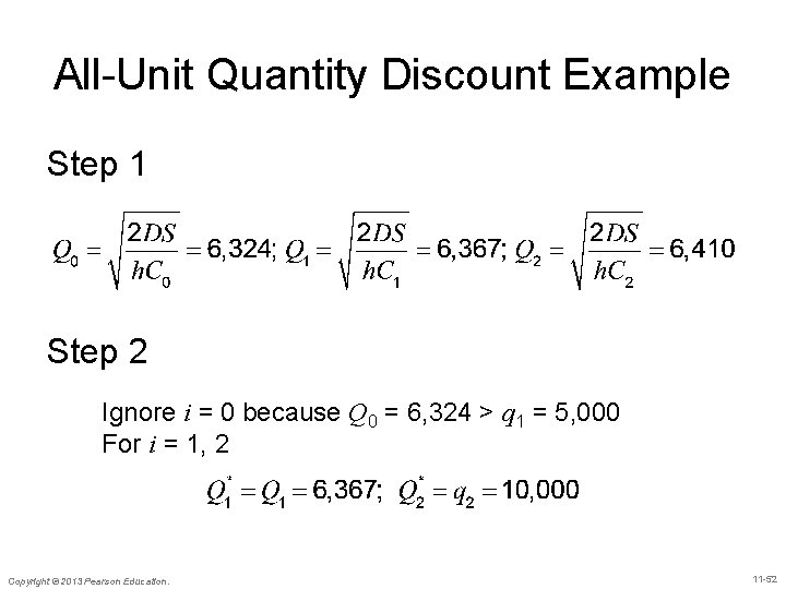
All-Unit Quantity Discount Example Step 1 Step 2 Ignore i = 0 because Q 0 = 6, 324 > q 1 = 5, 000 For i = 1, 2 Copyright © 2013 Pearson Education. 11 -52

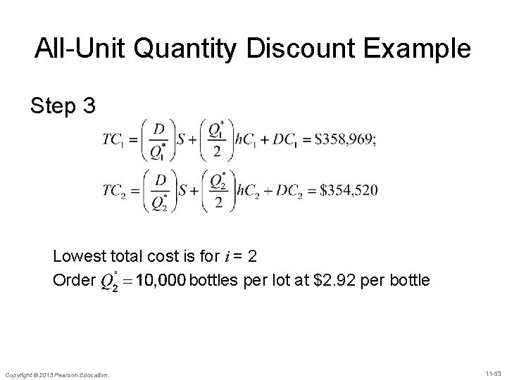
All-Unit Quantity Discount Example Step 3 Lowest total cost is for i = 2 Order bottles per lot at $2. 92 per bottle Copyright © 2013 Pearson Education. 11 -53

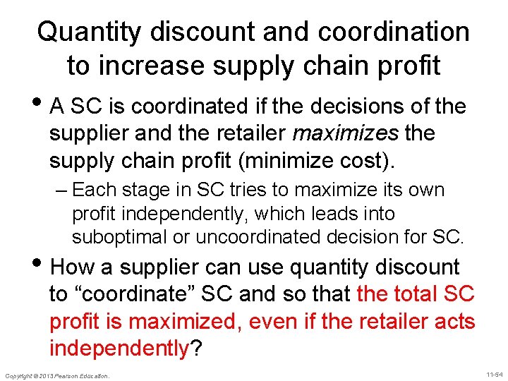
Quantity discount and coordination to increase supply chain profit • A SC is coordinated if the decisions of the supplier and the retailer maximizes the supply chain profit (minimize cost). – Each stage in SC tries to maximize its own profit independently, which leads into suboptimal or uncoordinated decision for SC. • How a supplier can use quantity discount to “coordinate” SC and so that the total SC profit is maximized, even if the retailer acts independently? Copyright © 2013 Pearson Education. 11 -54

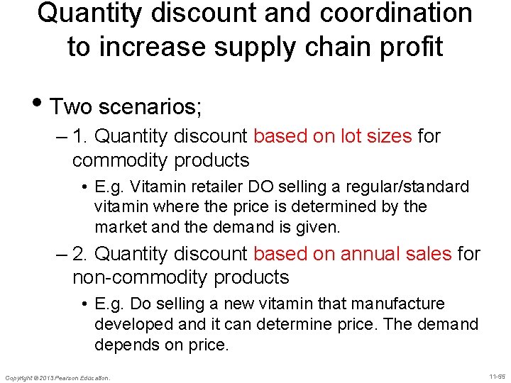
Quantity discount and coordination to increase supply chain profit • Two scenarios; – 1. Quantity discount based on lot sizes for commodity products • E. g. Vitamin retailer DO selling a regular/standard vitamin where the price is determined by the market and the demand is given. – 2. Quantity discount based on annual sales for non-commodity products • E. g. Do selling a new vitamin that manufacture developed and it can determine price. The demand depends on price. Copyright © 2013 Pearson Education. 11 -55

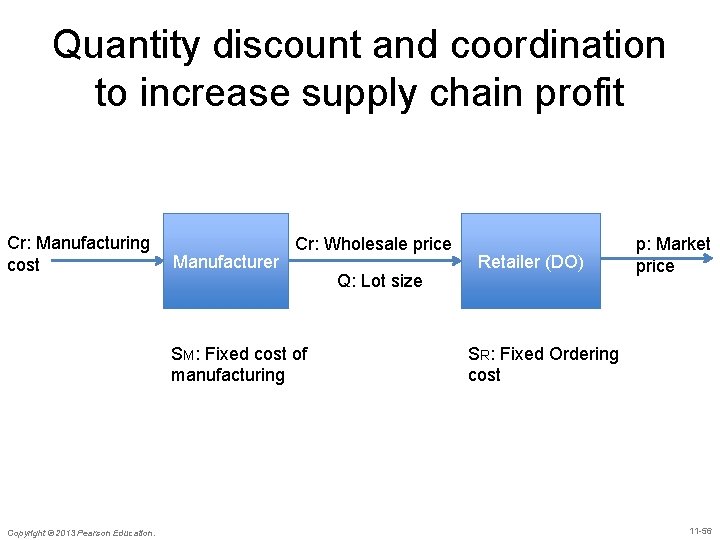
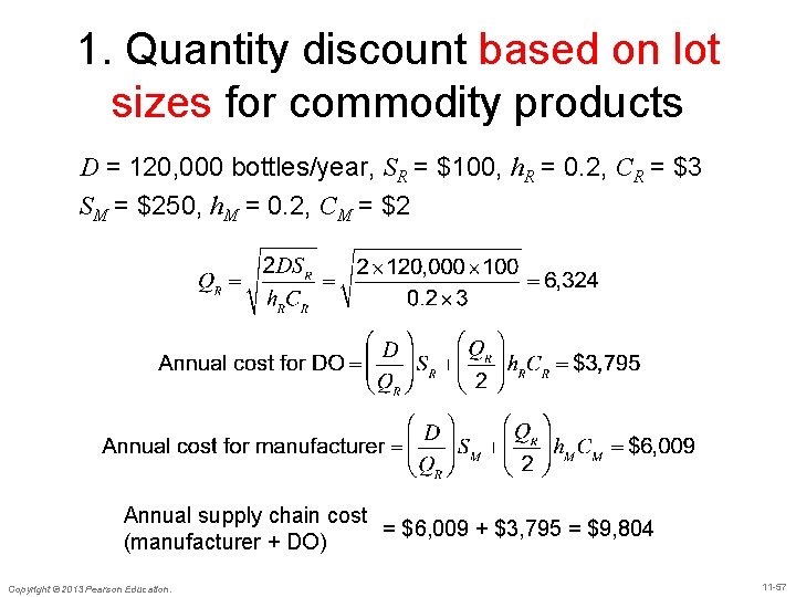
Quantity discount and coordination to increase supply chain profit Cr: Manufacturing cost Manufacturer Cr: Wholesale price SM: Fixed cost of manufacturing Copyright © 2013 Pearson Education. Q: Lot size Retailer (DO) p: Market price SR: Fixed Ordering cost 11 -56

1. Quantity discount based on lot sizes for commodity products D = 120, 000 bottles/year, SR = $100, h. R = 0. 2, CR = $3 SM = $250, h. M = 0. 2, CM = $2 Annual supply chain cost = $6, 009 + $3, 795 = $9, 804 (manufacturer + DO) Copyright © 2013 Pearson Education. 11 -57

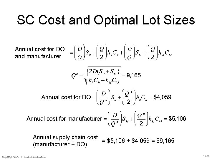
SC Cost and Optimal Lot Sizes Annual cost for DO and manufacturer Annual supply chain cost = $5, 106 + $4, 059 = $9, 165 (manufacturer + DO) Copyright © 2013 Pearson Education. 11 -58

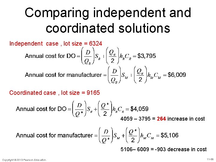
Comparing independent and coordinated solutions Independent case , lot size = 6324 Coordinated case , lot size = 9165 4059 – 3795 = 264 increase in cost 5106– 6009 = -903 decrease in cost Copyright © 2013 Pearson Education. 11 -59

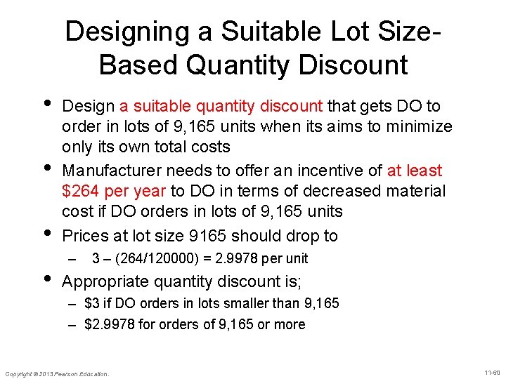
Designing a Suitable Lot Size. Based Quantity Discount • • Design a suitable quantity discount that gets DO to order in lots of 9, 165 units when its aims to minimize only its own total costs Manufacturer needs to offer an incentive of at least $264 per year to DO in terms of decreased material cost if DO orders in lots of 9, 165 units Prices at lot size 9165 should drop to – 3 – (264/120000) = 2. 9978 per unit Appropriate quantity discount is; – $3 if DO orders in lots smaller than 9, 165 – $2. 9978 for orders of 9, 165 or more Copyright © 2013 Pearson Education. 11 -60

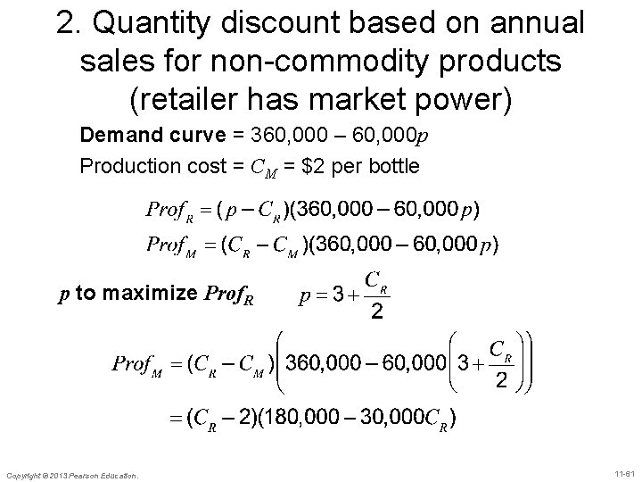
2. Quantity discount based on annual sales for non-commodity products (retailer has market power) Demand curve = 360, 000 – 60, 000 p Production cost = CM = $2 per bottle p to maximize Prof. R Copyright © 2013 Pearson Education. 11 -61

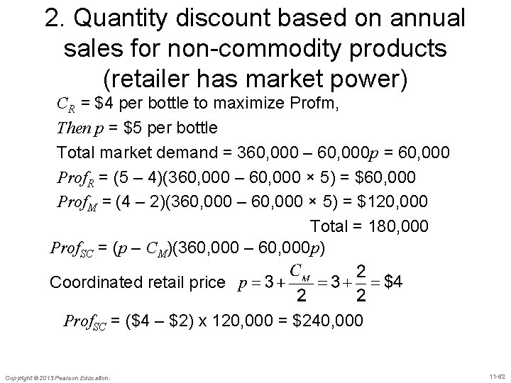
2. Quantity discount based on annual sales for non-commodity products (retailer has market power) CR = $4 per bottle to maximize Profm, Then p = $5 per bottle Total market demand = 360, 000 – 60, 000 p = 60, 000 Prof. R = (5 – 4)(360, 000 – 60, 000 × 5) = $60, 000 Prof. M = (4 – 2)(360, 000 – 60, 000 × 5) = $120, 000 Total = 180, 000 Prof. SC = (p – CM)(360, 000 – 60, 000 p) Coordinated retail price Prof. SC = ($4 – $2) x 120, 000 = $240, 000 Copyright © 2013 Pearson Education. 11 -62

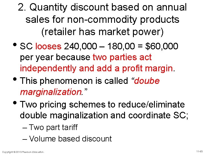
2. Quantity discount based on annual sales for non-commodity products (retailer has market power) • SC looses 240, 000 – 180, 00 = $60, 000 • • per year because two parties act independently and add a profit margin. This phenomenon is called “doube marginalization. ” Two pricing schemes to reduce/eliminate double maginalization and coordinate SC; – Two part tariff – Volume based discount Copyright © 2013 Pearson Education. 11 -63

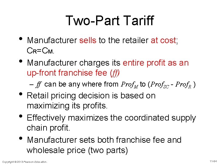
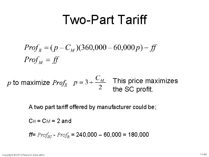
Two-Part Tariff • Manufacturer sells to the retailer at cost; • CR=CM. Manufacturer charges its entire profit as an up-front franchise fee (ff) – ff can be any where from Prof. M to (Prof. SC - Prof. R ) • Retail pricing decision is based on • • maximizing its profits. Effectively maximizes the coordinated supply chain profit. Manufacturer sets both franchise fee and wholesale price (two parts) Copyright © 2013 Pearson Education. 11 -64

Two-Part Tariff p to maximize Prof. R This price maximizes the SC profit. A two part tariff offered by manufacturer could be; CR = CM = 2 and ff= Prof. SC - Prof. R = 240, 000 – 60, 000 = 180, 000 Copyright © 2013 Pearson Education. 11 -65

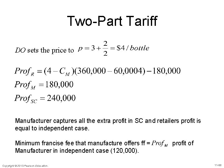
Two-Part Tariff DO sets the price to Manufacturer captures all the extra profit in SC and retailers profit is equal to independent case. Minimum francise fee that manufacture offers ff = Manufacturer in independent case (120, 000). Copyright © 2013 Pearson Education. profit of 11 -66

Volume-Based Quantity Discounts • Design a volume-based discount scheme that • • gets the retailer to purchase and sell the quantity sold when the two stages coordinate their actions. Lower price is offered for larger annual volumes. Two part tariff is effectively a volume based discount; Retailer’s effective price goes down as the purchased volume increases Copyright © 2013 Pearson Education. 11 -67

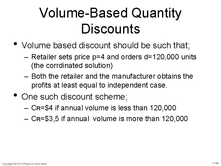
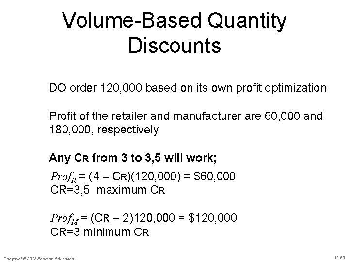
Volume-Based Quantity Discounts • Volume based discount should be such that; – Retailer sets price p=4 and orders d=120, 000 units (the corrdinated solution) – Both the retailer and the manufacturer obtains the profits at least equal to independent case. • One such discount scheme; – CR=$4 if annual volume is less than 120, 000 – CR=$3, 5 if annual volume is more than 120, 000 Copyright © 2013 Pearson Education. 11 -68

Volume-Based Quantity Discounts DO order 120, 000 based on its own profit optimization Profit of the retailer and manufacturer are 60, 000 and 180, 000, respectively Any CR from 3 to 3, 5 will work; Prof. R = (4 – CR)(120, 000) = $60, 000 CR=3, 5 maximum CR Prof. M = (CR – 2)120, 000 = $120, 000 CR=3 minimum CR Copyright © 2013 Pearson Education. 11 -69

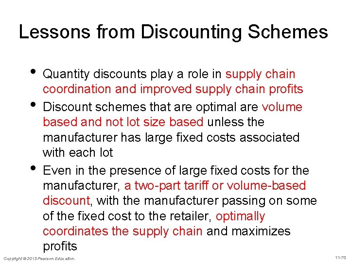
Lessons from Discounting Schemes • • • Quantity discounts play a role in supply chain coordination and improved supply chain profits Discount schemes that are optimal are volume based and not lot size based unless the manufacturer has large fixed costs associated with each lot Even in the presence of large fixed costs for the manufacturer, a two-part tariff or volume-based discount, with the manufacturer passing on some of the fixed cost to the retailer, optimally coordinates the supply chain and maximizes profits Copyright © 2013 Pearson Education. 11 -70

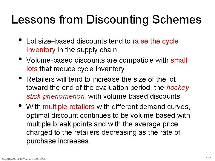
Lessons from Discounting Schemes • • Lot size–based discounts tend to raise the cycle inventory in the supply chain Volume-based discounts are compatible with small lots that reduce cycle inventory Retailers will tend to increase the size of the lot toward the end of the evaluation period, the hockey stick phenomenon, with volume based discounts With multiple retailers with different demand curves, optimal discount continues to be volume based with multiple break points and with the average price charged to the retailers decreasing as the rate of purchase increases. Copyright © 2013 Pearson Education. 11 -71

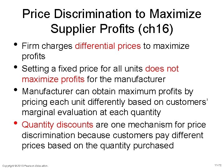
Price Discrimination to Maximize Supplier Profits (ch 16) • Firm charges differential prices to maximize • • • profits Setting a fixed price for all units does not maximize profits for the manufacturer Manufacturer can obtain maximum profits by pricing each unit differently based on customers’ marginal evaluation at each quantity Quantity discounts are one mechanism for price discrimination because customers pay different prices based on the quantity purchased Copyright © 2013 Pearson Education. 11 -72

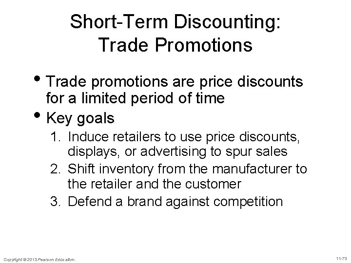
Short-Term Discounting: Trade Promotions • Trade promotions are price discounts • for a limited period of time Key goals 1. Induce retailers to use price discounts, displays, or advertising to spur sales 2. Shift inventory from the manufacturer to the retailer and the customer 3. Defend a brand against competition Copyright © 2013 Pearson Education. 11 -73

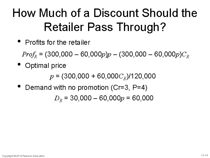
How Much of a Discount Should the Retailer Pass Through? • • • Profits for the retailer Prof. R = (300, 000 – 60, 000 p)p – (300, 000 – 60, 000 p)CR Optimal price p = (300, 000 + 60, 000 CR)/120, 000 Demand with no promotion (Cr=3, P=4) DR = 30, 000 – 60, 000 p = 60, 000 Copyright © 2013 Pearson Education. 11 -74

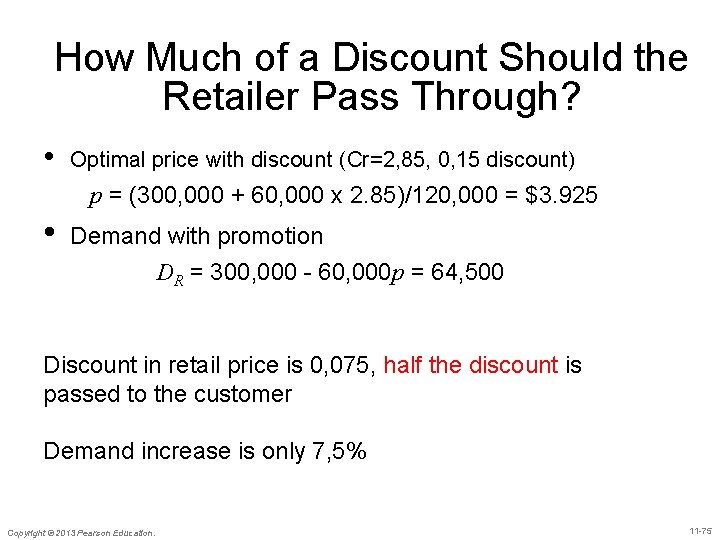
How Much of a Discount Should the Retailer Pass Through? • Optimal price with discount (Cr=2, 85, 0, 15 discount) p = (300, 000 + 60, 000 x 2. 85)/120, 000 = $3. 925 • Demand with promotion DR = 300, 000 - 60, 000 p = 64, 500 Discount in retail price is 0, 075, half the discount is passed to the customer Demand increase is only 7, 5% Copyright © 2013 Pearson Education. 11 -75

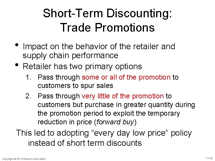
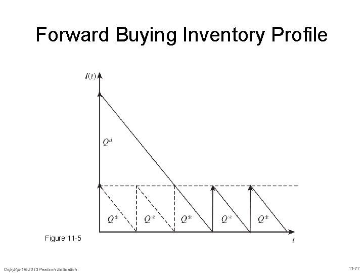
Short-Term Discounting: Trade Promotions • Impact on the behavior of the retailer and • supply chain performance Retailer has two primary options 1. Pass through some or all of the promotion to customers to spur sales 2. Pass through very little of the promotion to customers but purchase in greater quantity during the promotion period to exploit the temporary reduction in price (forward buy) This led to adopting “every day low price” policy instead of short term discounts Copyright © 2013 Pearson Education. 11 -76

Forward Buying Inventory Profile Figure 11 -5 Copyright © 2013 Pearson Education. 11 -77

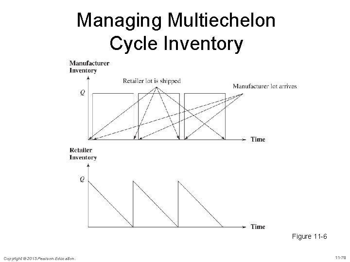
Managing Multiechelon Cycle Inventory • Multi-echelon supply chains have multiple • • stages with possibly many players at each stage Lack of coordination in lot sizing decisions across the supply chain results in high costs and more cycle inventory than required The goal is to decrease total costs by coordinating orders across the supply chain Copyright © 2013 Pearson Education. 11 -78

Managing Multiechelon Cycle Inventory Figure 11 -6 Copyright © 2013 Pearson Education. 11 -79

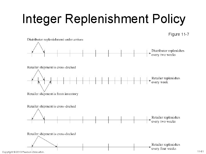
Integer Replenishment Policy • If one party in a supply chain supplies multiple parties at the next stage of SC; – Group the retailers based on their demand (low demad or high demand retailers) – All parties within a group order from the same supplier and have the same reorder interval. – Either retailers’ order frequency is an integer multiple of distributors order frequency or distributor’s order frequency is an integer multiple of retailers’ order frequency Copyright © 2013 Pearson Education. 11 -80

Integer Replenishment Policy Figure 11 -7 Copyright © 2013 Pearson Education. 11 -81

Integer Replenishment Policy • • Integer replenishment policy; every player applies a periodic replenishment policy and replenishment interval is an integer multiple of a base period (e. g. Week). Integer replenishment policy allows some part of the retailers order cross-docked (not waiting at the distributor) The relative frequency of reordering depends on the setup cost, holding cost, and demand at different parties These polices make the most sense for supply chains in which cycle inventories are large and demand is relatively predictable Copyright © 2013 Pearson Education. 11 -82

Summary of Learning Objectives 1. Balance the appropriate costs to choose the optimal lot size and cycle inventory in a supply chain 2. Understand the impact of quantity discounts on lot size and cycle inventory 3. Devise appropriate discounting schemes for a supply chain 4. Understand the impact of trade promotions on lot size and cycle inventory Copyright © 2013 Pearson Education. 11 -83

Summary of Learning Objectives 5. Identify managerial levers that reduce lot size and cycle inventory in a supply chain without increasing cost – Reduce fixed ordering and transportation costs incurred per order – Implement volume-based discounting schemes rather than individual lot size–based discounting schemes – Eliminate or reduce trade promotions and encourage EDLP – base trade promotions on sellthrough rather than sell-in to the retailer Copyright © 2013 Pearson Education. 11 -84

All rights reserved. No part of this publication may be reproduced, stored in a retrieval system, or transmitted, in any form or by any means, electronic, mechanical, photocopying, recording, or otherwise, without the prior written permission of the publisher. Printed in the United States of America. Copyright © 2013 Pearson Education. 11 -85