Vehicle Routing John H Vande Vate Fall 2002

Vehicle Routing John H. Vande Vate Fall, 2002 1 1

Shared Transportation Capacity • Large shipments reduce transportation costs but increase inventory costs • EOQ trades off these two costs • Reduce shipment size without increasing transportation costs? • Combine shipments on one vehicle 2 2

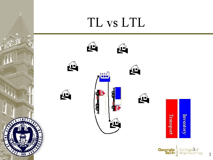
TL vs LTL Transport Inventory 3 3

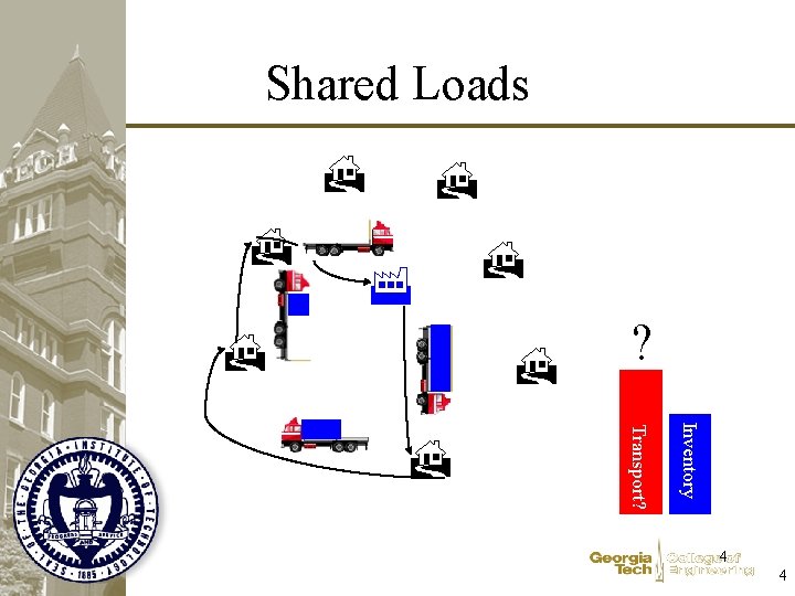
Shared Loads Transport? Inventory ? 4 4

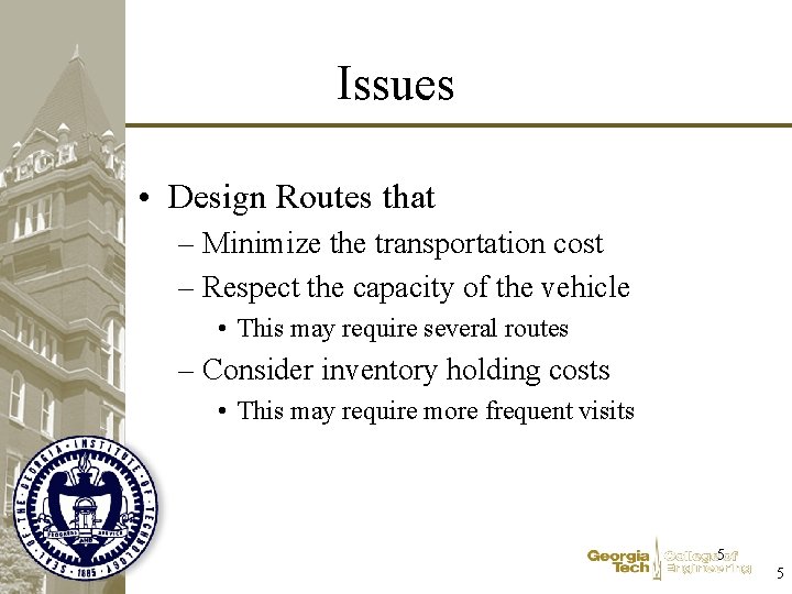
Issues • Design Routes that – Minimize the transportation cost – Respect the capacity of the vehicle • This may require several routes – Consider inventory holding costs • This may require more frequent visits 5 5

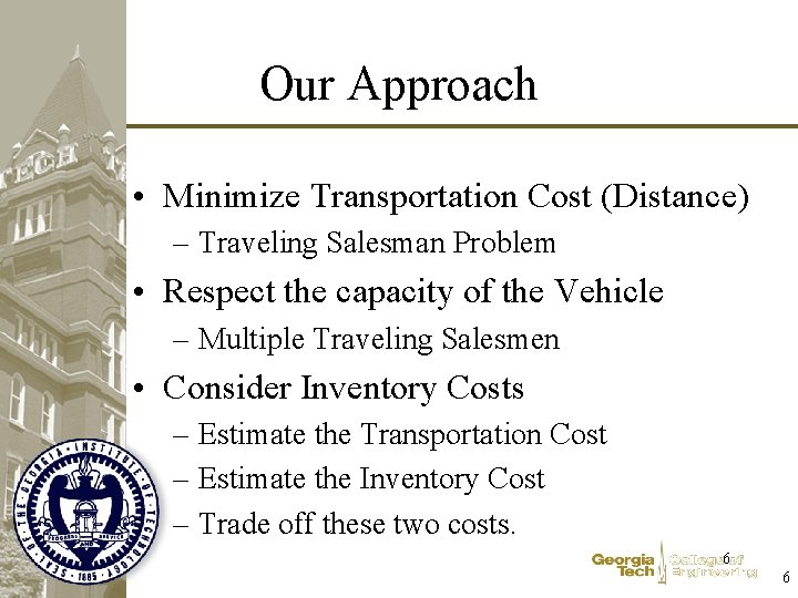
Our Approach • Minimize Transportation Cost (Distance) – Traveling Salesman Problem • Respect the capacity of the Vehicle – Multiple Traveling Salesmen • Consider Inventory Costs – Estimate the Transportation Cost – Estimate the Inventory Cost – Trade off these two costs. 6 6

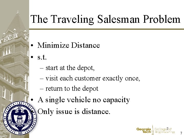
The Traveling Salesman Problem • Minimize Distance • s. t. – start at the depot, – visit each customer exactly once, – return to the depot • A single vehicle no capacity • Only issue is distance. 7 7

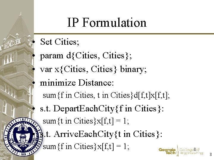
IP Formulation • • Set Cities; param d{Cities, Cities}; var x{Cities, Cities} binary; minimize Distance: sum{f in Cities, t in Cities}d[f, t]x[f, t]; • s. t. Depart. Each. City{f in Cities}: sum{t in Cities}x[f, t] = 1; • s. t. Arrive. Each. City{t in Cities}: sum{f in Cities}x[f, t] = 1; 8 8

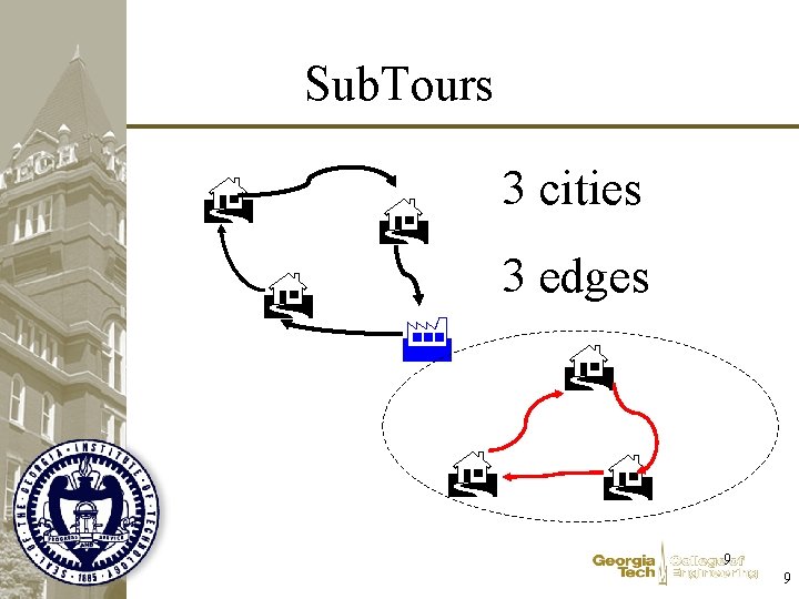
Sub. Tours 3 cities 3 edges 9 9

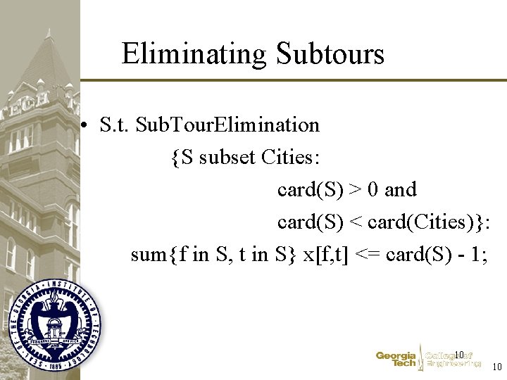
Eliminating Subtours • S. t. Sub. Tour. Elimination {S subset Cities: card(S) > 0 and card(S) < card(Cities)}: sum{f in S, t in S} x[f, t] <= card(S) - 1; 10 10

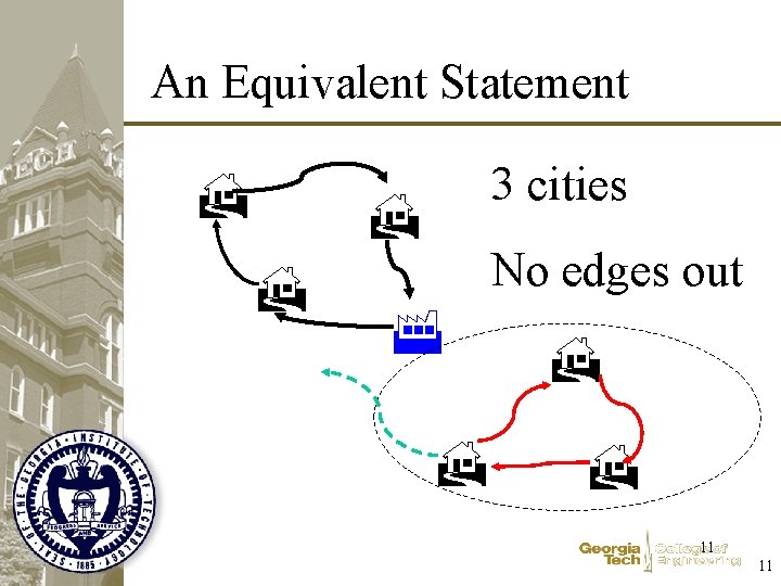
An Equivalent Statement 3 cities No edges out 11 11

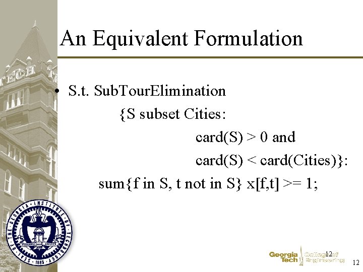
An Equivalent Formulation • S. t. Sub. Tour. Elimination {S subset Cities: card(S) > 0 and card(S) < card(Cities)}: sum{f in S, t not in S} x[f, t] >= 1; 12 12

How Many Constraints? • How many subsets of N items? • 2 N • Omit 2 subsets: – All N items – The empty set • 2 N - 2 13 13

OK, Half of that. . . • If we have an edge out of S, we must have an edge out of NS. • Why? The edge out of S is an edge into NS. But there are exactly |NS| edges into cities in NS. Since one of them comes from S, not all the edges from cities in NS can lead to cities in NS. At least one must go to S. 14 14

Still Lots! • How many subsets of N items? • 2 N • Omit 2 subsets: – All N items – The empty set • 2 N - 2 • Half of that: 2 N-1 - 1 15 15

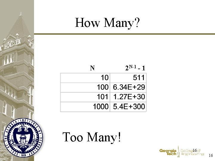
How Many? N 2 N-1 - 1 Too Many! 16 16

Optimization is Possible But. . . • • It is difficult Few 100 cities is the limit Is it appropriate? Other approaches…. 17 17

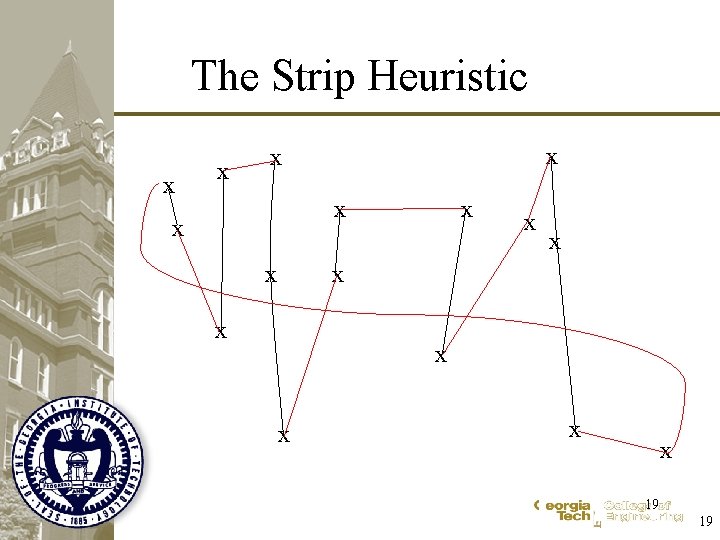
Heuristics • The Strip Heuristic – Partition the region into narrow strips – Routing in each strip is easy ~ 1 -Dimensional – Paste the routes together 18 18

The Strip Heuristic x x x x 19 19

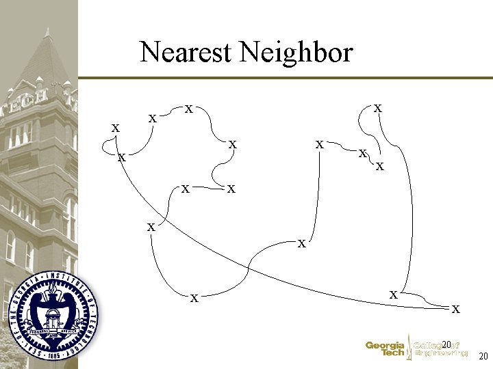
Nearest Neighbor x x x x 20 20

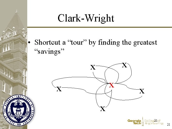
Clark-Wright • Shortcut a “tour” by finding the greatest “savings” x x x 21 21

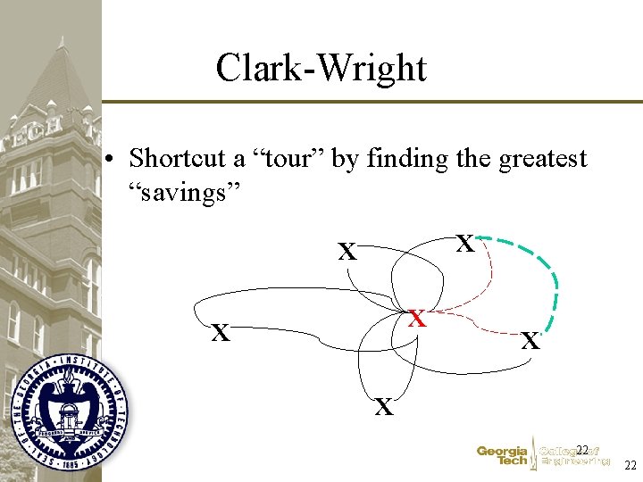
Clark-Wright • Shortcut a “tour” by finding the greatest “savings” x x x 22 22

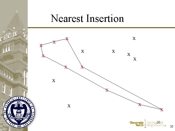
Nearest Insertion x x x x 23 23

Nearest Insertion x x x x 24 24

Nearest Insertion x x x x 25 25

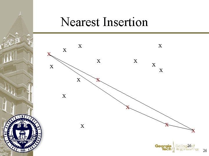
Nearest Insertion x x x x 26 26

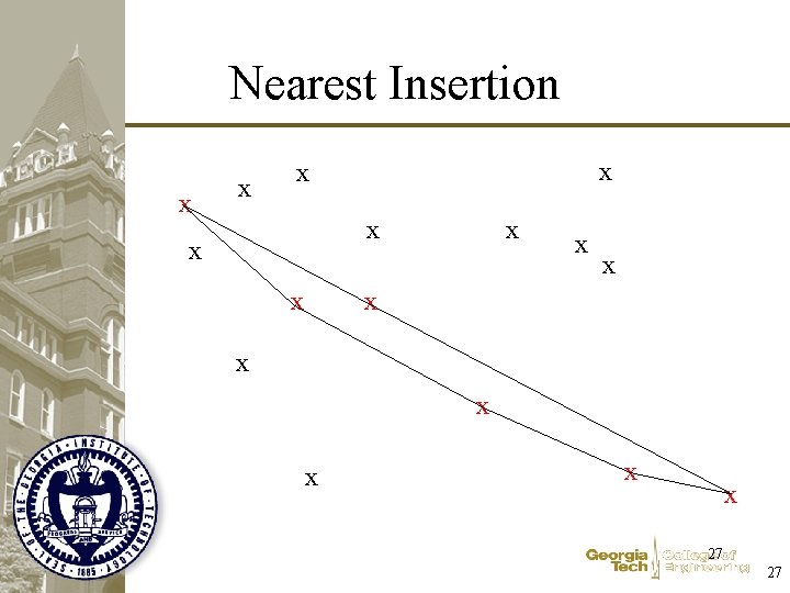
Nearest Insertion x x x x 27 27

Nearest Insertion x x x x 28 28

Nearest Insertion x x x x 29 29

Nearest Insertion x x x x 30 30

Nearest Insertion x x x x 31 31

Nearest Insertion x x x x 32 32

Nearest Insertion x x x x 33 33

Nearest Insertion x x x x 34 34

Nearest Insertion x x x x 35 35

Nearest Insertion x x x x 36 36

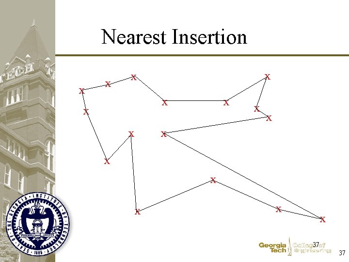
Nearest Insertion x x x x 37 37

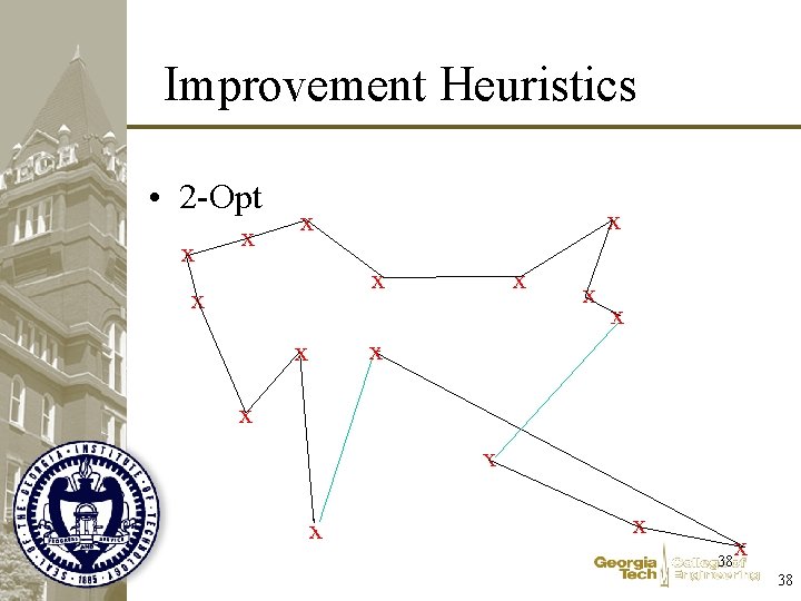
Improvement Heuristics • 2 -Opt x x x x 38

Local Minima • No improvement found, but… • Tour still isn’t good 39 39

Probabilistic Methods • Simulated Annealing • With probability that reduces over time, accept an exchange that makes things worse (gets you out of local minima). 40 40

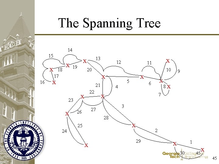
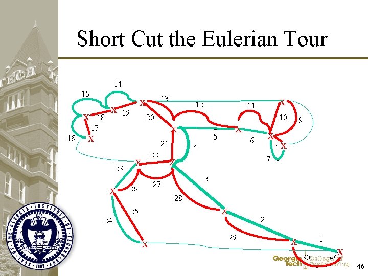
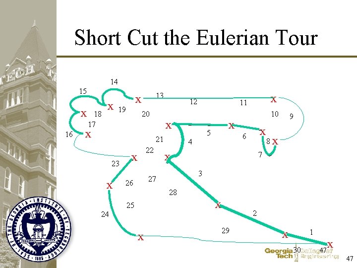
Optimization-Based Heuristics • Minimum Spanning Tree Heuristic • Build a minimum spanning tree on the edges between customers • Double the tree to get an Eulerian Tour (visits everyone perhaps several times and returns to the start) • Short cut the Eulerian Tour to get a Hamilton Tour (Traveling Salesman Tour) 41 41

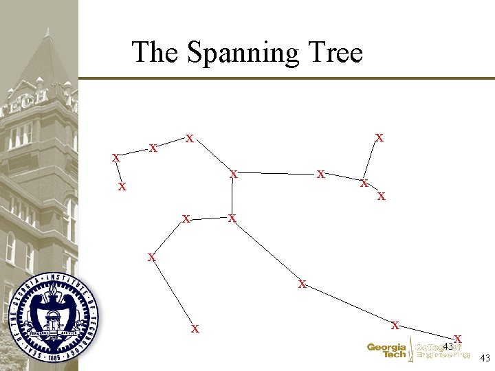
The Spanning Tree • Is Easy to construct – Use the Greedy Algorithm • Add edges in increasing order of length • Discard any that create a cycle • Is a Lower bound on the TSP – Drop one edge from the TSP and you have a spanning tree – It must be at least as long as the minimum spanning tree 42 42

The Spanning Tree x x x x 43

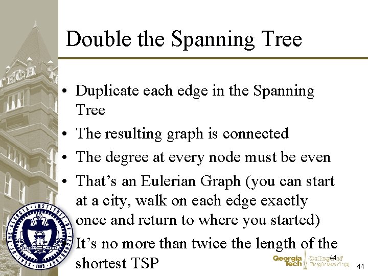
Double the Spanning Tree • Duplicate each edge in the Spanning Tree • The resulting graph is connected • The degree at every node must be even • That’s an Eulerian Graph (you can start at a city, walk on each edge exactly once and return to where you started) • It’s no more than twice the length of the 44 shortest TSP 44

The Spanning Tree 14 15 x 16 18 17 x 13 x 19 20 x 12 x 21 23 x 24 22 x 10 x 5 x 6 4 x 9 8 x 7 3 27 26 x 11 28 x 25 x 2 29 x 1 30 45 x 45

Short Cut the Eulerian Tour 14 15 x 16 18 17 x 13 x 19 20 x 12 x 21 23 x 24 22 x 10 x 5 x 6 4 x 9 8 x 7 3 27 26 x 11 28 x 25 x 2 29 x 1 30 46 x 46

Short Cut the Eulerian Tour 14 15 x 16 18 17 x 13 x 19 20 x 12 x 21 23 x 24 22 x 10 x 5 x 6 4 x 9 8 x 7 3 27 26 x 11 28 x 25 x 2 29 x 1 30 47 x 47

Spacefilling Curves • There are no more points in the unit square than in the interval from 0 to 1!? 48 48

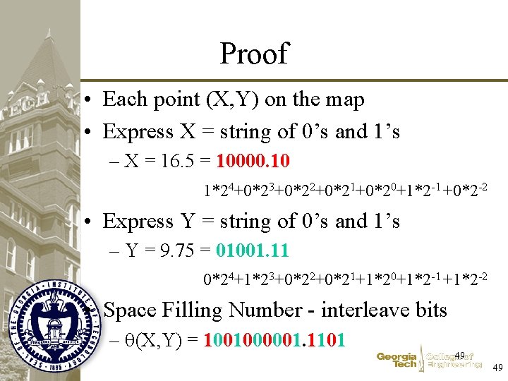
Proof • Each point (X, Y) on the map • Express X = string of 0’s and 1’s – X = 16. 5 = 10000. 10 1*24+0*23+0*22+0*21+0*20+1*2 -1 +0*2 -2 • Express Y = string of 0’s and 1’s – Y = 9. 75 = 01001. 11 0*24+1*23+0*22+0*21+1*20+1*2 -1 +1*2 -2 • Space Filling Number - interleave bits – (X, Y) = 1001000001. 1101 49 49

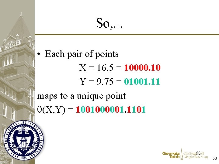
So, . . . • Each pair of points X = 16. 5 = 10000. 10 Y = 9. 75 = 01001. 11 maps to a unique point (X, Y) = 1001000001. 1101 50 50

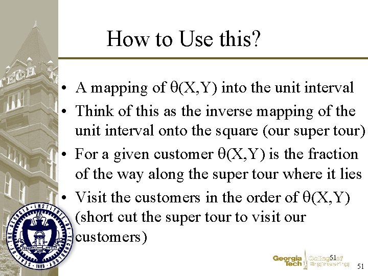
How to Use this? • A mapping of (X, Y) into the unit interval • Think of this as the inverse mapping of the unit interval onto the square (our super tour) • For a given customer (X, Y) is the fraction of the way along the super tour where it lies • Visit the customers in the order of (X, Y) (short cut the super tour to visit our customers) 51 51

The TSP • For More on Space. Filling Curves visit http: //www. isye. gatech. edu/faculty/John_Bartholdi/mow. html • There are several books on the TSP • …. 52 52

Our Approach • Minimize Transportation Cost (Distance) – Traveling Salesman Problem • Respect the capacity of the Vehicle – Multiple Traveling Salesmen • Consider Inventory Costs – Estimate the Transportation Cost – Estimate the Inventory Cost – Trade off these two costs. 53 53

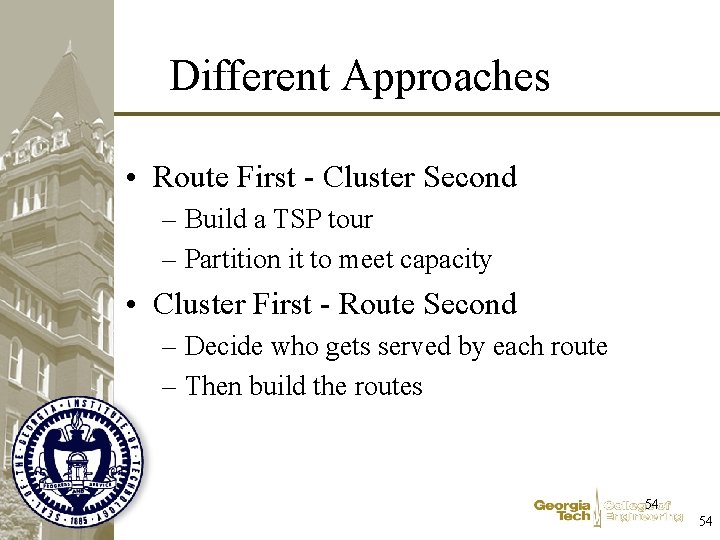
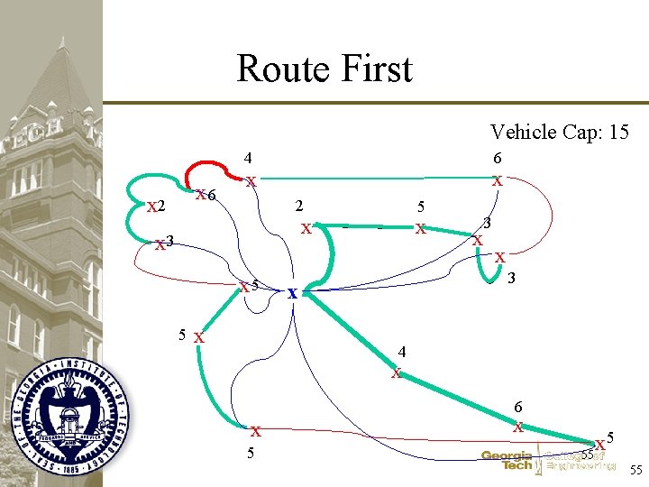
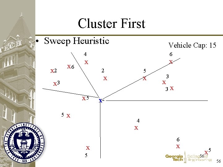
Different Approaches • Route First - Cluster Second – Build a TSP tour – Partition it to meet capacity • Cluster First - Route Second – Decide who gets served by each route – Then build the routes 54 54

Route First Vehicle Cap: 15 6 4 x 6 x 2 x x 2 5 x x 3 x 5 5 x x x 3 x 4 x 6 x 5 x 55 55

Cluster First • Sweep Heuristic Vehicle Cap: 15 6 4 x 6 x 2 x x 2 5 x x 3 3 x 5 5 x x x 4 x 6 x 5 x 56 56

Our Approach • Minimize Transportation Cost (Distance) – Traveling Salesman Problem • Respect the capacity of the Vehicle – Multiple Traveling Salesmen • Consider Inventory Costs – Estimate the Transportation Cost – Estimate the Inventory Cost – Trade off these two costs. 57 57