Transportation Model Lecture 16 Dr Arshad Zaheer Source

Transportation Model Lecture 16 Dr. Arshad Zaheer Source: Operations Research- An Introduction by Hamdy A. Taha, 8 th edition

Simplex Algorithm – Special cases • There are four special cases arise in the use of the simplex method. 1. 2. 3. 4. Degeneracy Alternative optimal Unbounded solution infeasible solution 2

Outline q What is transportation model q Purpose of Transportation Model q Real Life Application q Explanation of Transportation model q Formulating a transportation problem q. Finding the initial feasible solution

What is Transportation model? q The transportation problem is one of the subclasses of linear programming problem where the objective is to transport various quantities of a single homogeneous product that are initially stored at various origins, to different destinations in such a way that the total transportation is minimum.

Purpose of Transportation models q Transportation models or problems are primarily concerned with the optimal (best possible) way in which a product produced at different factories or plants (called supply origins) can be transported to a number of warehouses (called demand destinations). q The objective in a transportation problem is to fully satisfy the destination requirements within the operating production capacity constraints at the minimum possible cost.

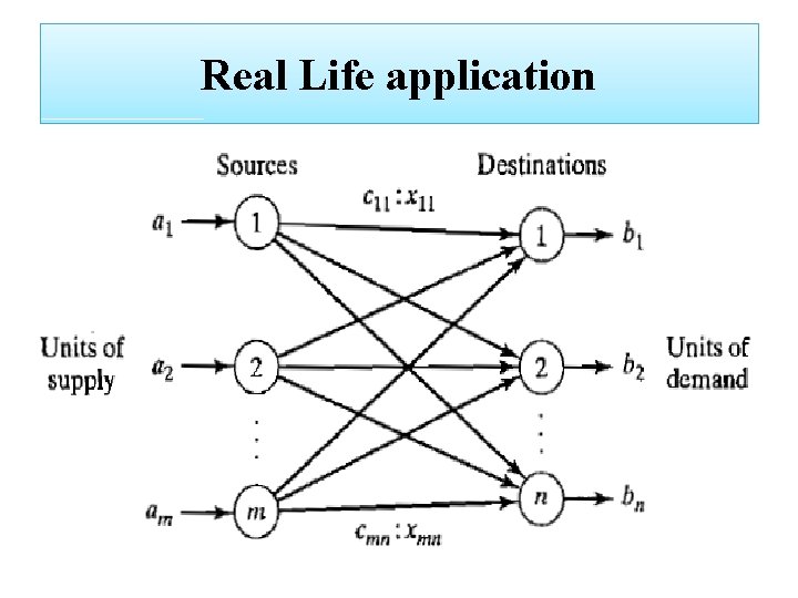
Real Life application

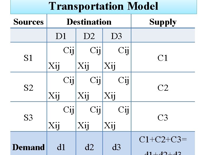
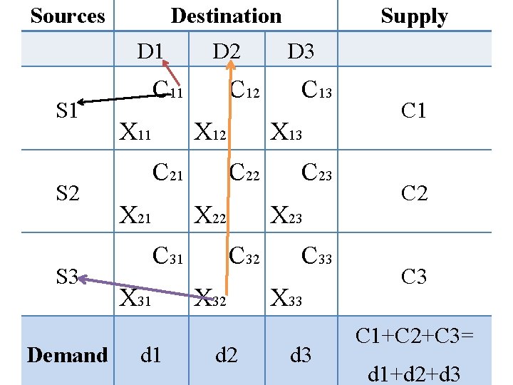
Transportation Model Sources Destination D 1 S 2 S 3 Demand D 2 Cij Xij Cij Cij d 1 Cij Xij Xij D 3 Cij Xij Supply Cij Xij d 2 Cij Xij d 3 C 1 C 2 C 3 C 1+C 2+C 3=

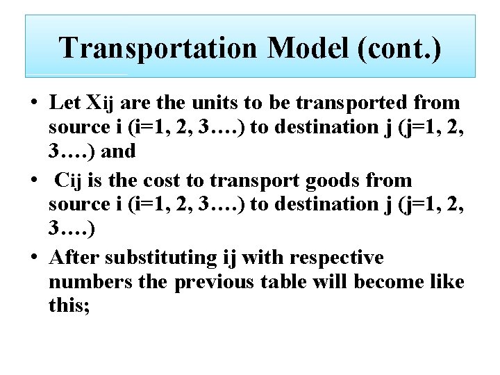
Transportation Model (cont. ) • Let Xij are the units to be transported from source i (i=1, 2, 3…. ) to destination j (j=1, 2, 3…. ) and • Cij is the cost to transport goods from source i (i=1, 2, 3…. ) to destination j (j=1, 2, 3…. ) • After substituting ij with respective numbers the previous table will become like this;

Sources Destination D 1 S 2 S 3 Demand D 2 C 11 X 11 C 12 X 12 C 21 X 22 X 31 d 1 D 3 C 13 X 13 C 22 C 31 Supply C 23 X 23 C 32 X 32 d 2 C 33 X 33 d 3 C 1 C 2 C 3 C 1+C 2+C 3= d 1+d 2+d 3

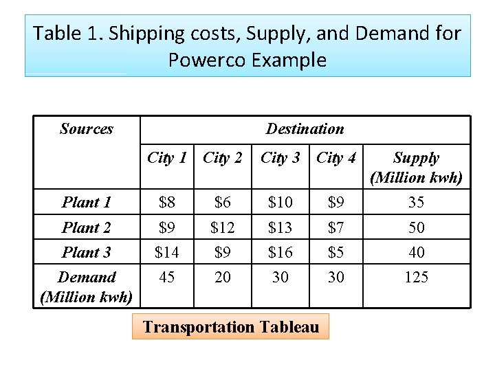
Formulating Transportation Problems Lets take an example to describe the procedure of formulation of problem; Example 1: Powerco has three electric power plants that supply the electric needs of four cities. q The associated supply of each plant and demand of each city is given in the table 1.

Table 1. Shipping costs, Supply, and Demand for Powerco Example Sources Destination City 1 City 2 City 3 City 4 Supply (Million kwh) Plant 1 $8 $6 $10 $9 35 Plant 2 Plant 3 Demand (Million kwh) $9 $14 45 $12 $9 20 $13 $16 30 $7 $5 30 50 40 125 Transportation Tableau

Formulating Transportation Problems (Cont. ) A transportation problem is specified by the supply, the demand, and the shipping costs. So the relevant data can be summarized in a transportation tableau. The transportation tableau implicitly expresses the supply and demand constraints and the shipping cost between each demand supply point.

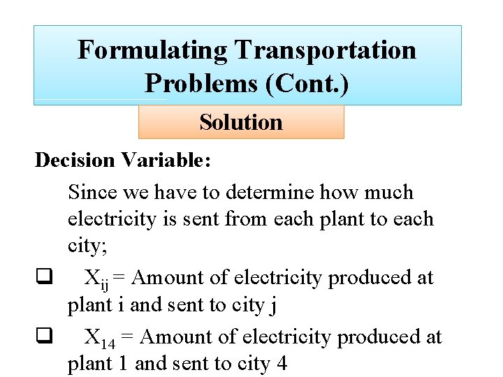
Formulating Transportation Problems (Cont. ) Solution Decision Variable: Since we have to determine how much electricity is sent from each plant to each city; q Xij = Amount of electricity produced at plant i and sent to city j q X 14 = Amount of electricity produced at plant 1 and sent to city 4

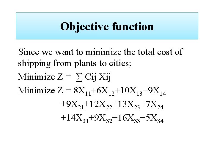
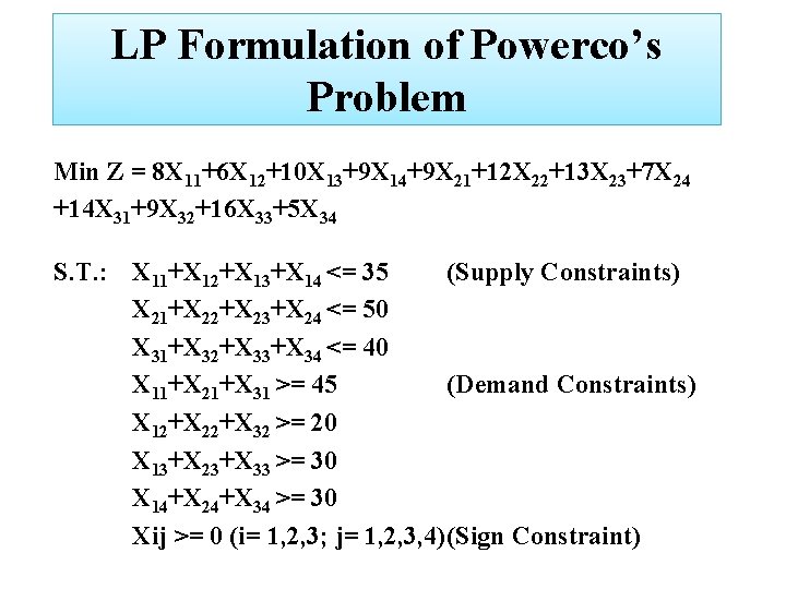
Objective function Since we want to minimize the total cost of shipping from plants to cities; Minimize Z = ∑ Cij Xij Minimize Z = 8 X 11+6 X 12+10 X 13+9 X 14 +9 X 21+12 X 22+13 X 23+7 X 24 +14 X 31+9 X 32+16 X 33+5 X 34

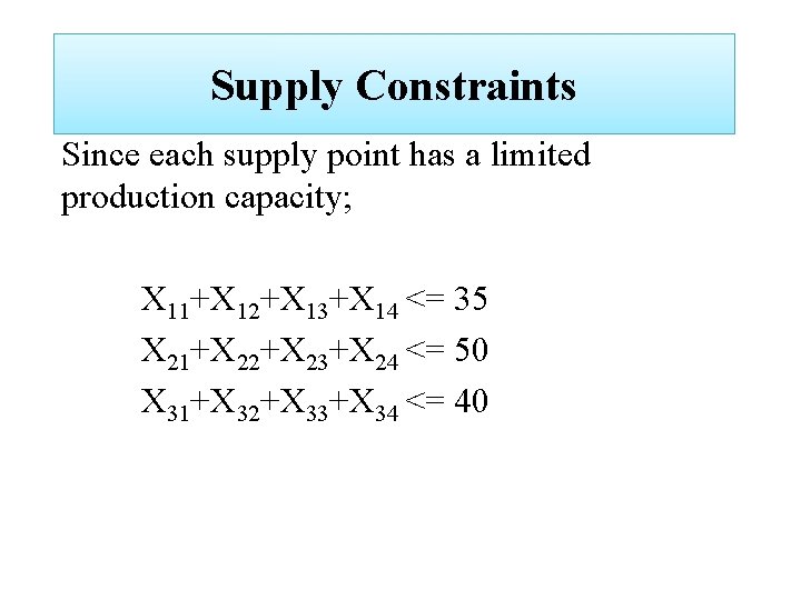
Supply Constraints Since each supply point has a limited production capacity; X 11+X 12+X 13+X 14 <= 35 X 21+X 22+X 23+X 24 <= 50 X 31+X 32+X 33+X 34 <= 40

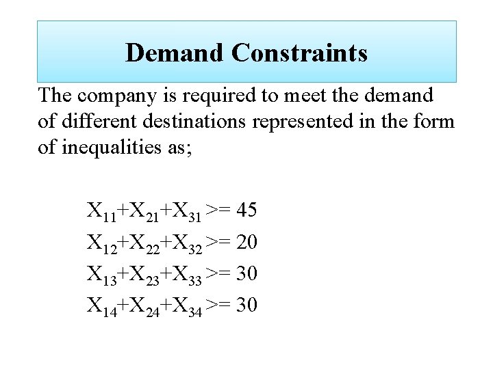
Demand Constraints The company is required to meet the demand of different destinations represented in the form of inequalities as; X 11+X 21+X 31 >= 45 X 12+X 22+X 32 >= 20 X 13+X 23+X 33 >= 30 X 14+X 24+X 34 >= 30

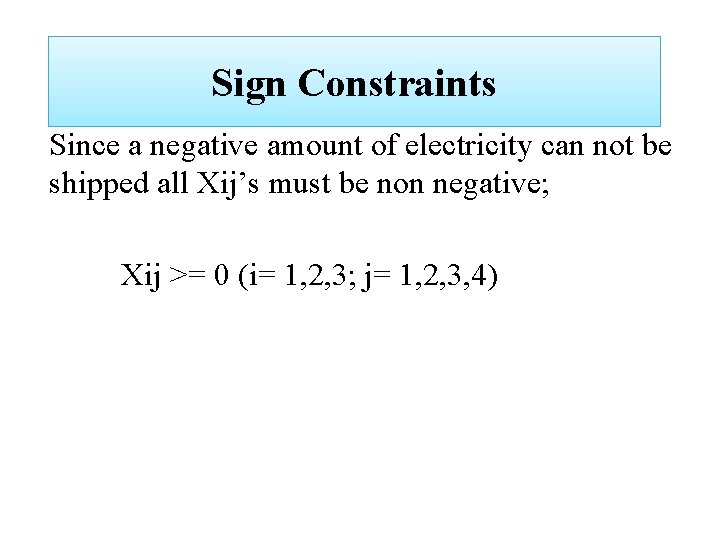
Sign Constraints Since a negative amount of electricity can not be shipped all Xij’s must be non negative; Xij >= 0 (i= 1, 2, 3; j= 1, 2, 3, 4)

LP Formulation of Powerco’s Problem Min Z = 8 X 11+6 X 12+10 X 13+9 X 14+9 X 21+12 X 22+13 X 23+7 X 24 +14 X 31+9 X 32+16 X 33+5 X 34 S. T. : X 11+X 12+X 13+X 14 <= 35 (Supply Constraints) X 21+X 22+X 23+X 24 <= 50 X 31+X 32+X 33+X 34 <= 40 X 11+X 21+X 31 >= 45 (Demand Constraints) X 12+X 22+X 32 >= 20 X 13+X 23+X 33 >= 30 X 14+X 24+X 34 >= 30 Xij >= 0 (i= 1, 2, 3; j= 1, 2, 3, 4)(Sign Constraint)

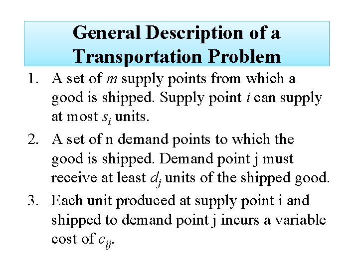
General Description of a Transportation Problem 1. A set of m supply points from which a good is shipped. Supply point i can supply at most si units. 2. A set of n demand points to which the good is shipped. Demand point j must receive at least dj units of the shipped good. 3. Each unit produced at supply point i and shipped to demand point j incurs a variable cost of cij.

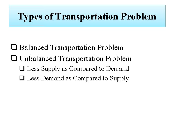
Types of Transportation Problem q Balanced Transportation Problem q Unbalanced Transportation Problem q Less Supply as Compared to Demand q Less Demand as Compared to Supply

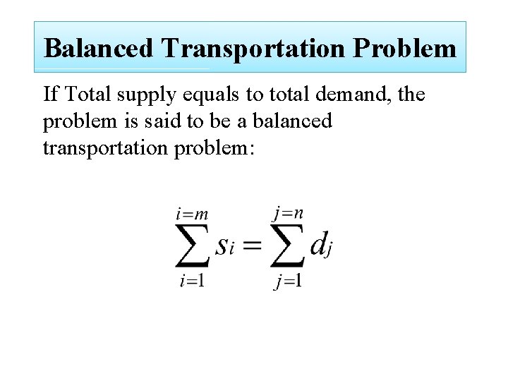
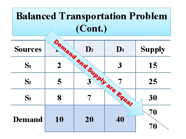
Balanced Transportation Problem If Total supply equals to total demand, the problem is said to be a balanced transportation problem:

Balanced Transportation Problem (Cont. ) D Sources em D 1 an d S 1 2 S 2 5 S 3 Demand 8 10 D 2 an d 4 S up pl 3 y 7 20 ar e D 3 Supply 3 15 7 25 Eq 3 ua l 40 30 70 70

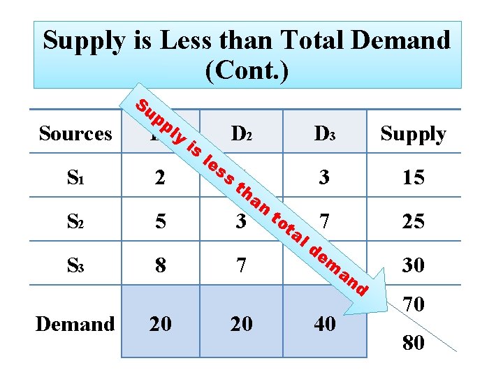
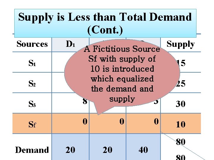
Supply is Less than Total Demand If a transportation problem has a total supply that is strictly less than total demand the problem has no feasible solution. There is no doubt that in such a case one or more of the demand will be left unmet. Generally in such situations a penalty cost is often associated with unmet demand as one can guess this time the total penalty cost is desired to be minimum. To solve such problem we need to introduce fictitious sources to provide the required supply at zero cost or cost provided in the problem.

Supply is Less than Total Demand (Cont. ) Su Sources pp D 1 ly S 1 2 S 2 5 3 S 3 8 7 Demand 20 is le D 2 ss t 4 h an 20 D 3 Supply 3 15 to ta 7 ld em 3 25 an d 40 30 70 80

Supply is Less than Total Demand (Cont. ) Sources D 1 D 2 D 3 S 3 A Fictitious Source of 3 2 Sf with supply 4 10 is introduced 5 which equalized 3 7 the demand supply 8 7 3 Sf 0 S 1 S 2 Demand 20 0 40 Supply 15 25 30 10 80

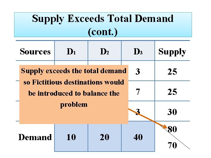
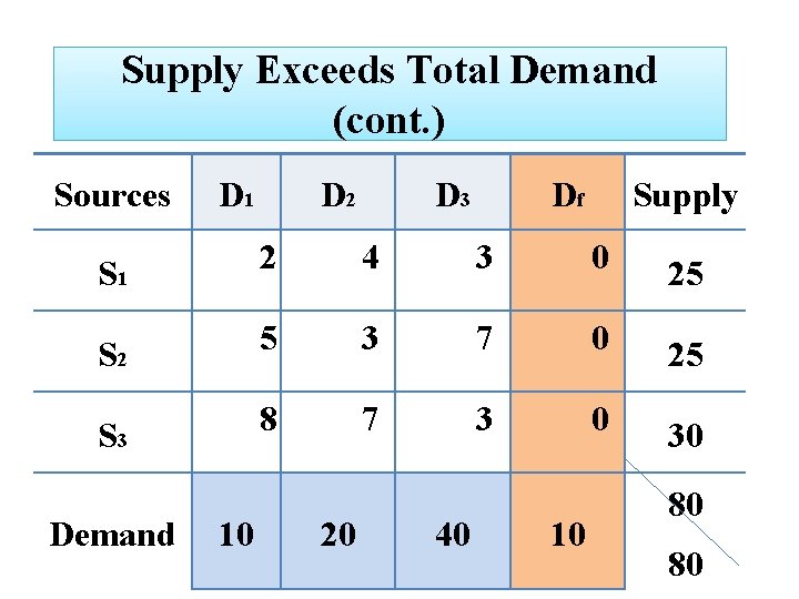
Supply Exceeds Total Demand If total supply exceeds total demand, we can balance the problem by adding dummy demand point. Since shipments to the dummy demand point are not real, they are assigned a cost of zero.

Supply Exceeds Total Demand (cont. ) Sources D 1 D 2 D 3 Supply S 1 exceeds 2 the total demand 4 3 so Fictitious destinations would 3 the 7 be. S 2 introduced 5 to balance problem S 3 8 7 3 Demand 10 20 40 Supply 25 25 30 80 70

Supply Exceeds Total Demand (cont. ) Sources D 1 D 2 D 3 Df Supply S 1 2 4 3 0 25 S 2 5 3 7 0 25 S 3 8 7 3 0 30 Demand 10 20 40 10 80 80

Initial Feasible Solution Unlike other Linear Programming problems, a balanced TP with m supply points and n demand points is easier to solve, although it has m + n equality constraints. The reason for that is, if a set of decision variables (xij’s) satisfy all but one constraint, the values for xij’s will satisfy that remaining constraint automatically.

Methods to find Initial Feasible Solution There are two basic methods: 1. Northwest Corner Method 2. Least - Cost Method

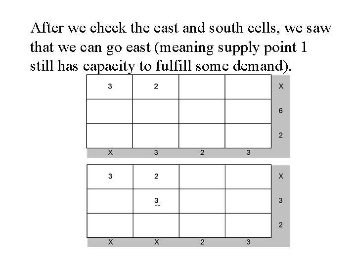
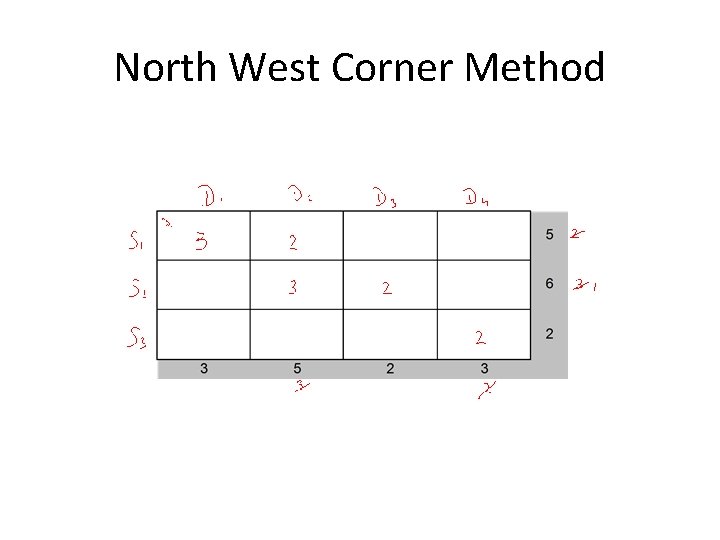
Northwest Corner Method To find the Initial Feasible Solution by the NWC method: Begin in the upper left (northwest) corner of the transportation tableau and set x 11 as large as possible (here the limitations for setting x 11 to a larger number, will be the demand of demand point 1 and the supply of supply point 1. Your x 11 value can not be greater than minimum of this 2 values).

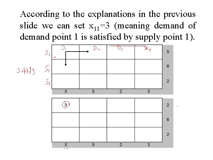
According to the explanations in the previous slide we can set x 11=3 (meaning demand of demand point 1 is satisfied by supply point 1).

After we check the east and south cells, we saw that we can go east (meaning supply point 1 still has capacity to fulfill some demand).

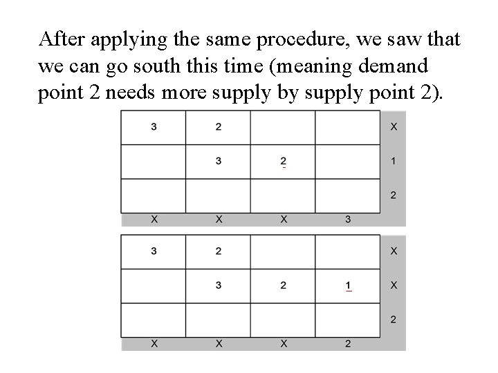
After applying the same procedure, we saw that we can go south this time (meaning demand point 2 needs more supply by supply point 2).

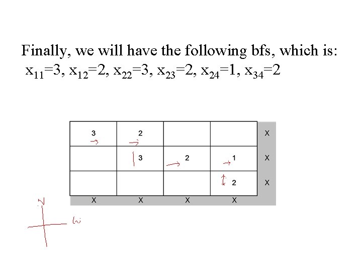
Finally, we will have the following bfs, which is: x 11=3, x 12=2, x 22=3, x 23=2, x 24=1, x 34=2

North West Corner Method

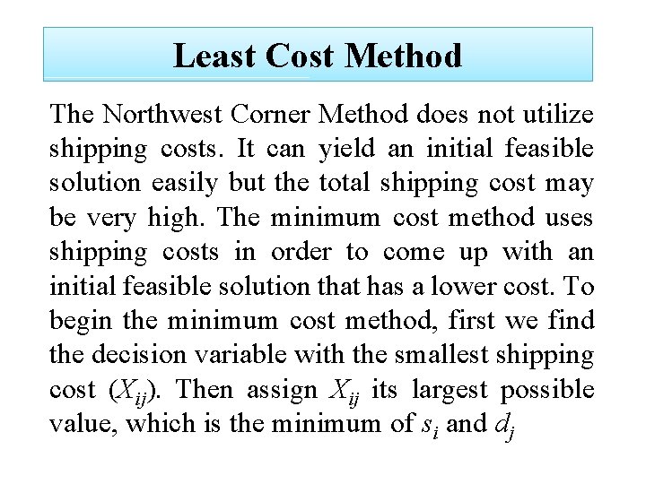
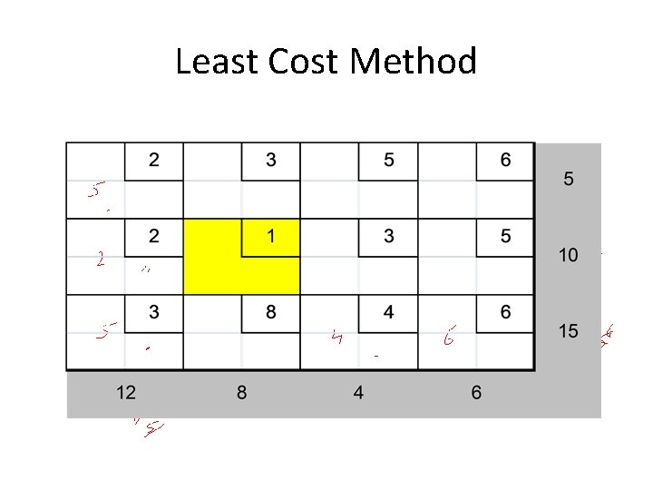
Least Cost Method The Northwest Corner Method does not utilize shipping costs. It can yield an initial feasible solution easily but the total shipping cost may be very high. The minimum cost method uses shipping costs in order to come up with an initial feasible solution that has a lower cost. To begin the minimum cost method, first we find the decision variable with the smallest shipping cost (Xij). Then assign Xij its largest possible value, which is the minimum of si and dj

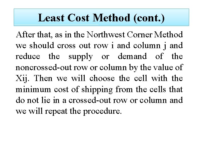
Least Cost Method (cont. ) After that, as in the Northwest Corner Method we should cross out row i and column j and reduce the supply or demand of the noncrossed-out row or column by the value of Xij. Then we will choose the cell with the minimum cost of shipping from the cells that do not lie in a crossed-out row or column and we will repeat the procedure.

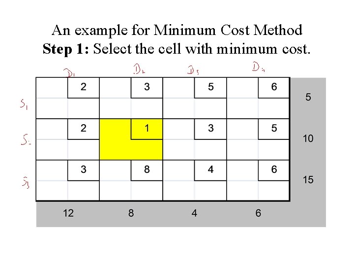
An example for Minimum Cost Method Step 1: Select the cell with minimum cost.

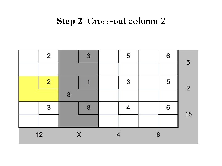
Step 2: Cross-out column 2

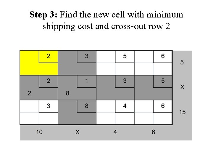
Step 3: Find the new cell with minimum shipping cost and cross-out row 2

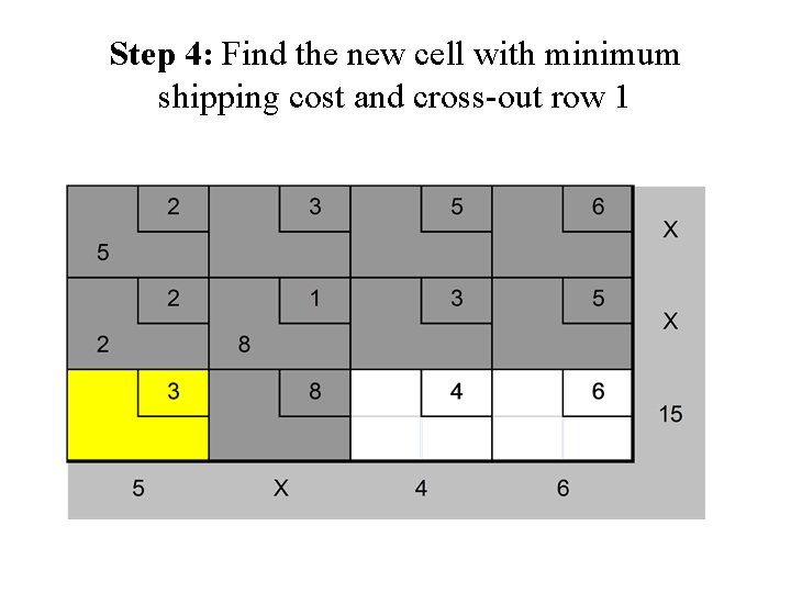
Step 4: Find the new cell with minimum shipping cost and cross-out row 1

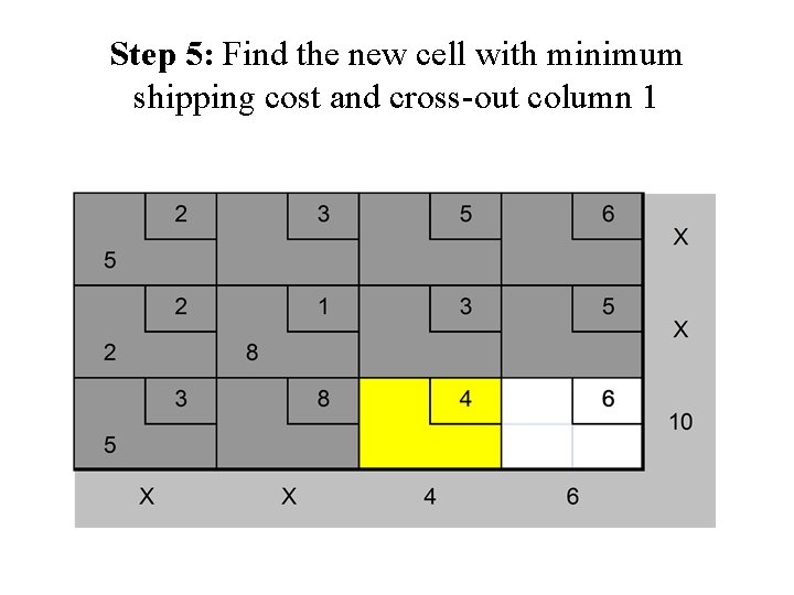
Step 5: Find the new cell with minimum shipping cost and cross-out column 1

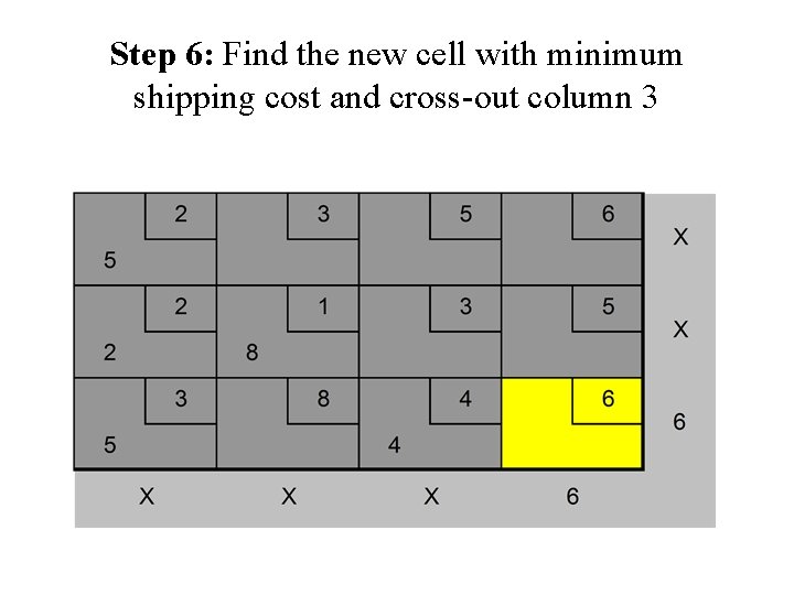
Step 6: Find the new cell with minimum shipping cost and cross-out column 3

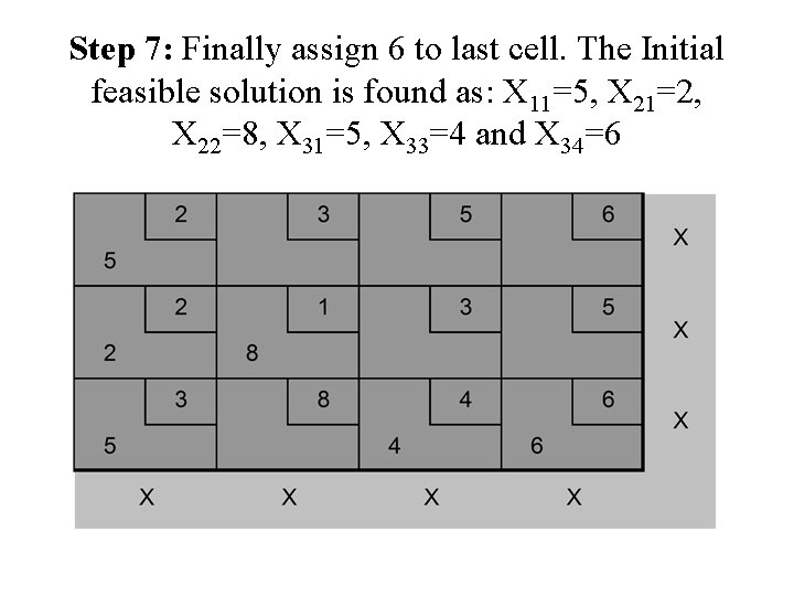
Step 7: Finally assign 6 to last cell. The Initial feasible solution is found as: X 11=5, X 21=2, X 22=8, X 31=5, X 33=4 and X 34=6

Least Cost Method