Transformations and Fitting EECS 442 Prof David Fouhey


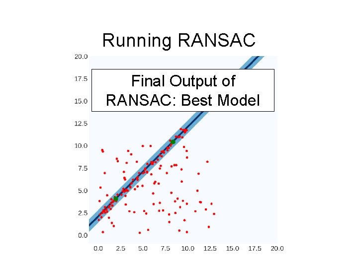
![Running RANSAC Point/line distance |n. T[x, y] – d| Trial #1 Best Model: None Running RANSAC Point/line distance |n. T[x, y] – d| Trial #1 Best Model: None](https://slidetodoc.com/presentation_image_h2/ad1127fd351aeefe2384aeae6fc2a870/image-37.jpg)
- Slides: 69

Transformations and Fitting EECS 442 – Prof. David Fouhey Winter 2019, University of Michigan http: //web. eecs. umich. edu/~fouhey/teaching/EECS 442_W 19/

Administrivia • Grading ~80% done • I will post a link to sign up for Amazon AWS resources. • Please sign up ASAP

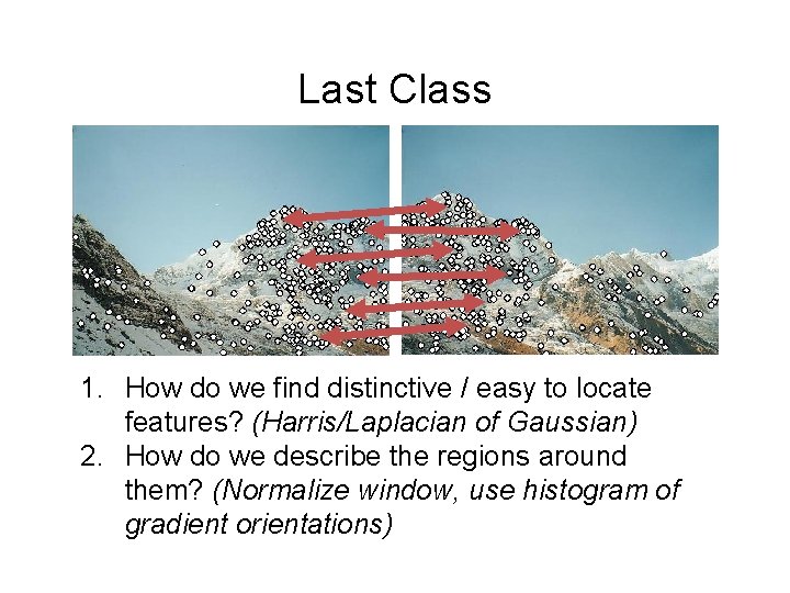
Last Class 1. How do we find distinctive / easy to locate features? (Harris/Laplacian of Gaussian) 2. How do we describe the regions around them? (Normalize window, use histogram of gradient orientations)

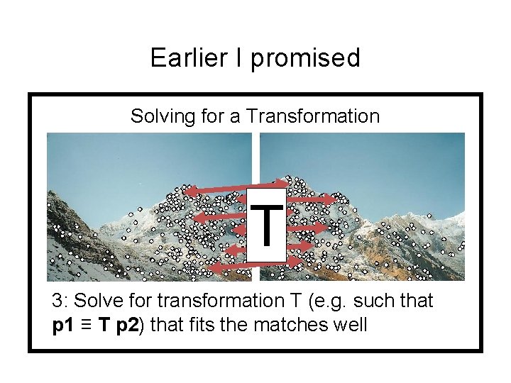
Earlier I promised Solving for a Transformation T 3: Solve for transformation T (e. g. such that p 1 ≡ T p 2) that fits the matches well

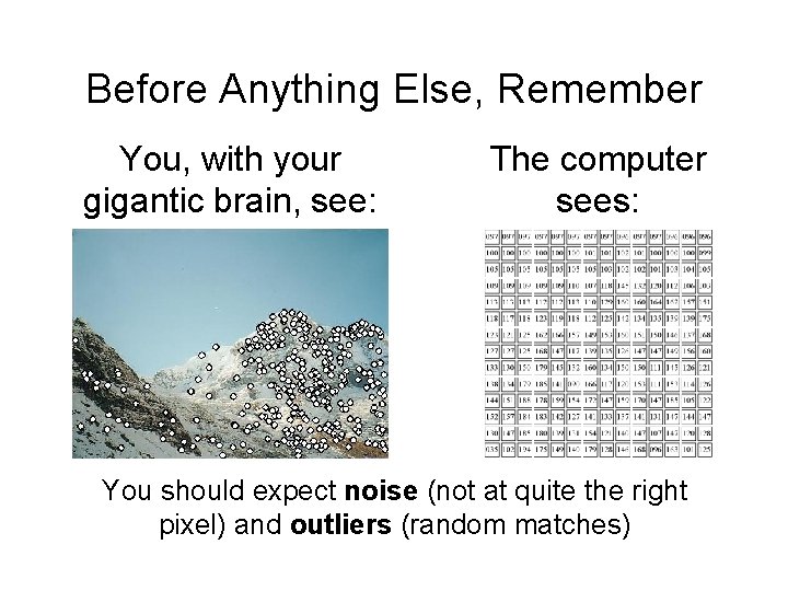
Before Anything Else, Remember You, with your gigantic brain, see: The computer sees: You should expect noise (not at quite the right pixel) and outliers (random matches)

Today • How do we fit models (i. e. , a parameteric representation of data that’s smaller than the data) to data? • How do we handle: • Noise – least squares / total least squares • Outliers – RANSAC (random sample consensus) • Multiple models – Hough Transform (can also make RANSAC handle this with some effort)

Working Example: Lines • We’ll handle lines as our models today since you should be familiar with them • Next class will cover more complex models. I promise we’ll eventually stitch images together • You can apply today’s techniques on next class’s models

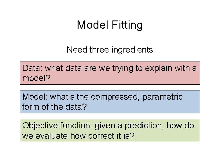
Model Fitting Need three ingredients Data: what data are we trying to explain with a model? Model: what’s the compressed, parametric form of the data? Objective function: given a prediction, how do we evaluate how correct it is?

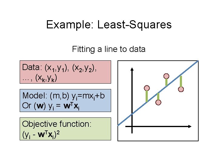
Example: Least-Squares Fitting a line to data Data: (x 1, y 1), (x 2, y 2), …, (xk, yk) Model: (m, b) yi=mxi+b Or (w) yi = w. Txi Objective function: (yi - w. Txi)2

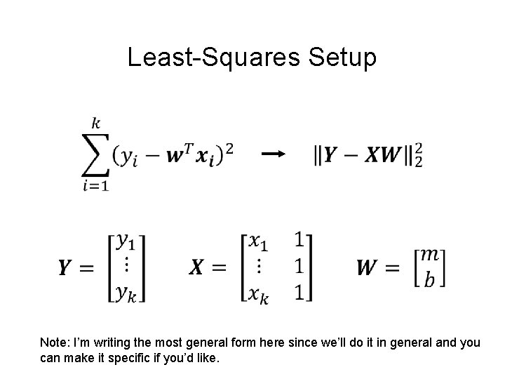
Least-Squares Setup Note: I’m writing the most general form here since we’ll do it in general and you can make it specific if you’d like.

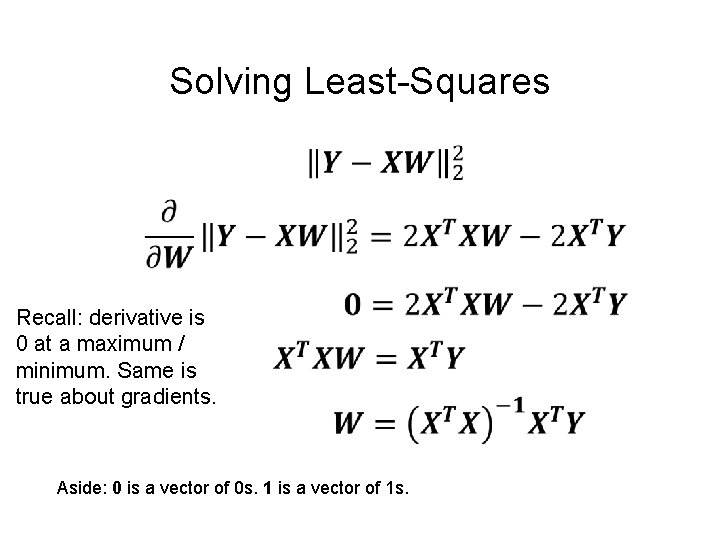
Solving Least-Squares Recall: derivative is 0 at a maximum / minimum. Same is true about gradients. Aside: 0 is a vector of 0 s. 1 is a vector of 1 s.

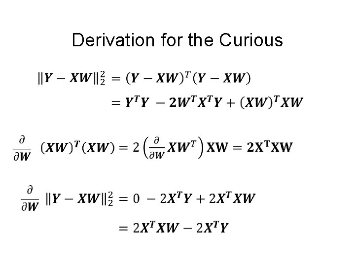
Derivation for the Curious

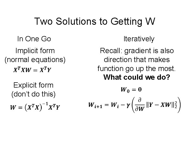
Two Solutions to Getting W In One Go Iteratively Implicit form (normal equations) Recall: gradient is also direction that makes function go up the most. What could we do? Explicit form (don’t do this)

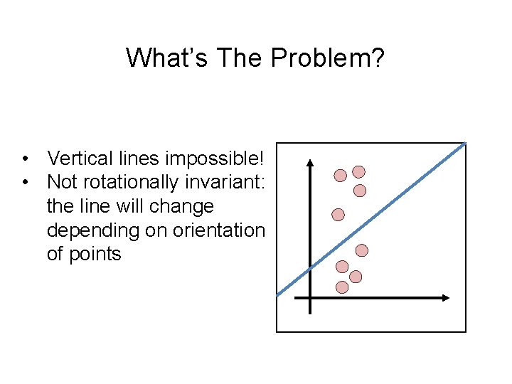
What’s The Problem? • Vertical lines impossible! • Not rotationally invariant: the line will change depending on orientation of points

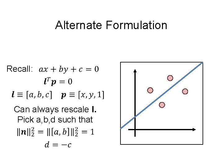
Alternate Formulation Recall: Can always rescale l. Pick a, b, d such that

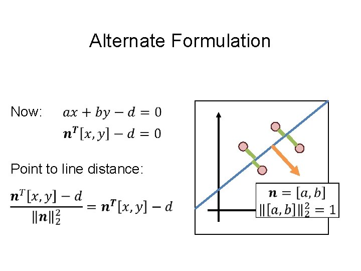
Alternate Formulation Now: Point to line distance:

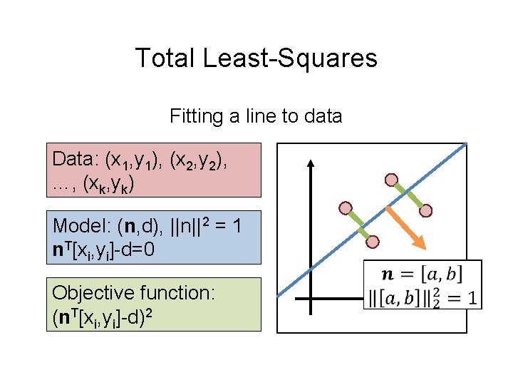
Total Least-Squares Fitting a line to data Data: (x 1, y 1), (x 2, y 2), …, (xk, yk) Model: (n, d), ||n||2 = 1 n. T[xi, yi]-d=0 Objective function: (n. T[xi, yi]-d)2

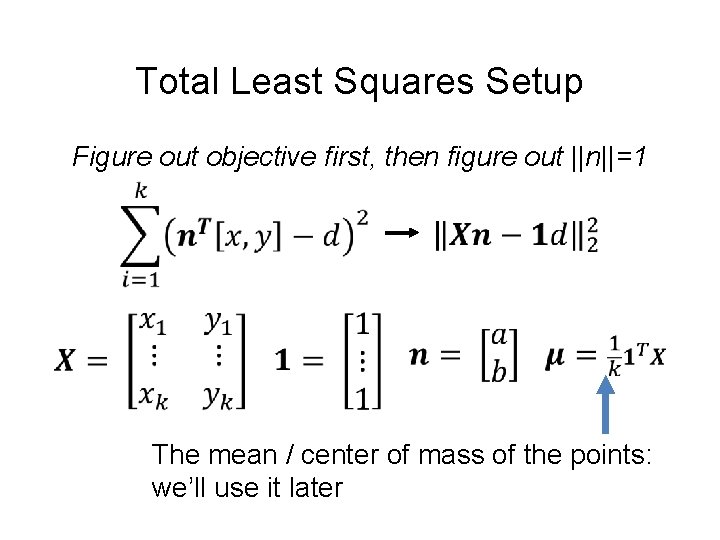
Total Least Squares Setup Figure out objective first, then figure out ||n||=1 The mean / center of mass of the points: we’ll use it later

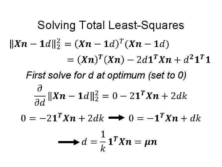
Solving Total Least-Squares First solve for d at optimum (set to 0)

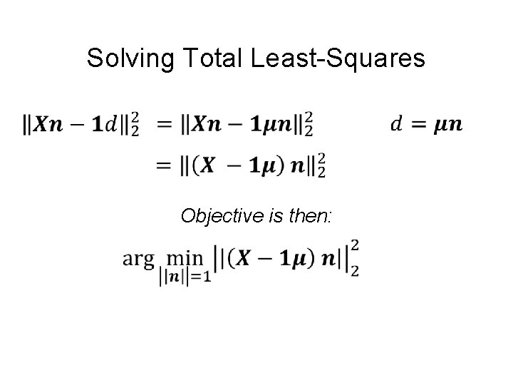
Solving Total Least-Squares Objective is then:

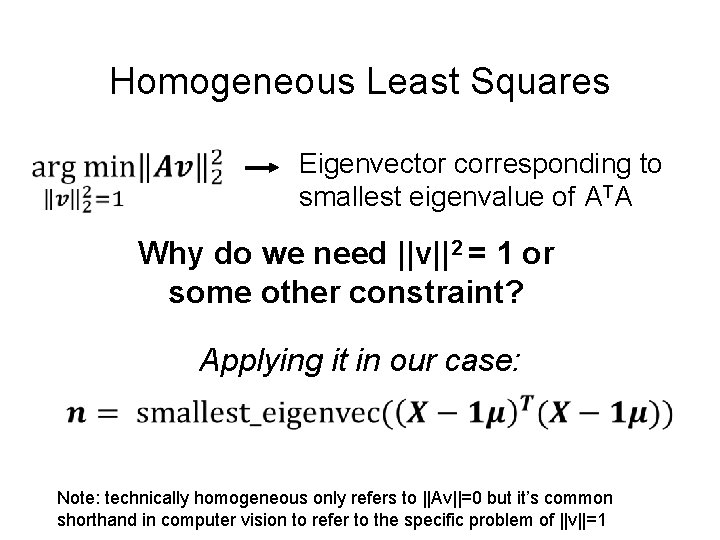
Homogeneous Least Squares Eigenvector corresponding to smallest eigenvalue of ATA Why do we need ||v||2 = 1 or some other constraint? Applying it in our case: Note: technically homogeneous only refers to ||Av||=0 but it’s common shorthand in computer vision to refer to the specific problem of ||v||=1

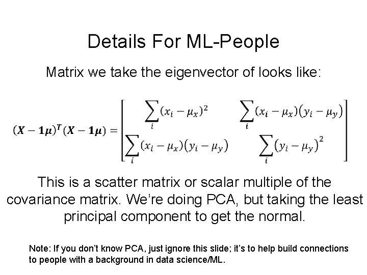
Details For ML-People Matrix we take the eigenvector of looks like: This is a scatter matrix or scalar multiple of the covariance matrix. We’re doing PCA, but taking the least principal component to get the normal. Note: If you don’t know PCA, just ignore this slide; it’s to help build connections to people with a background in data science/ML.

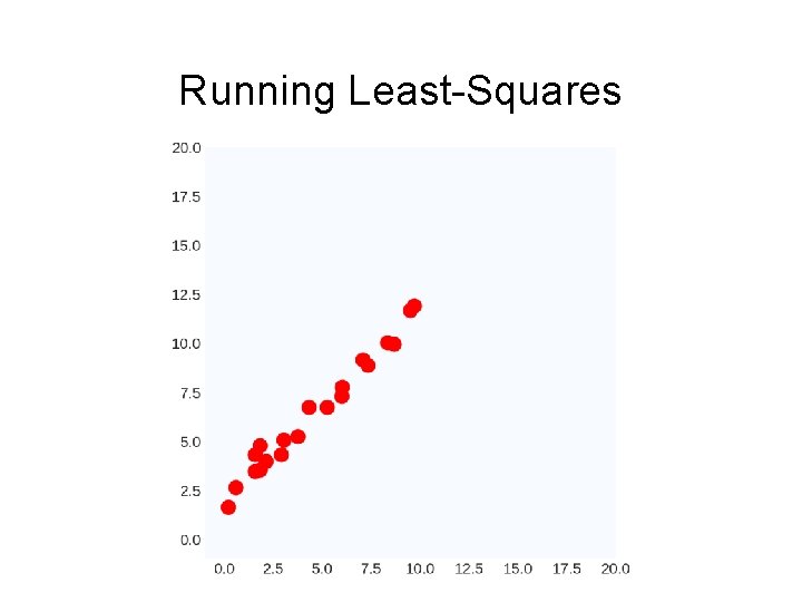
Running Least-Squares

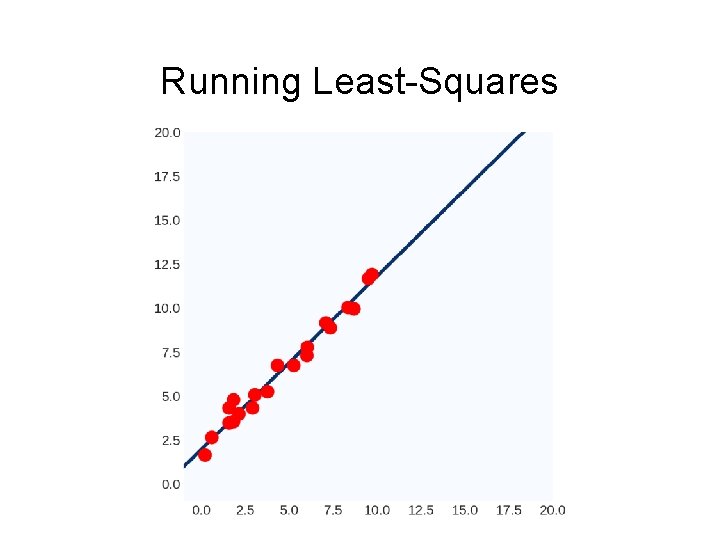
Running Least-Squares

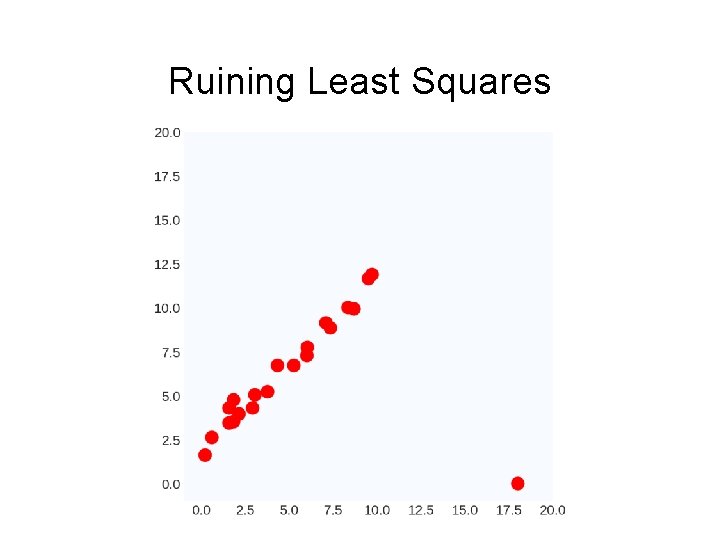
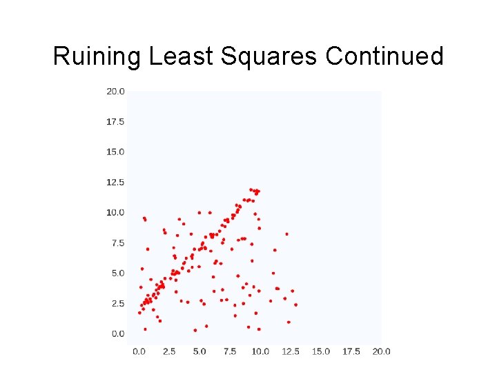
Ruining Least Squares

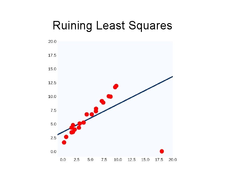
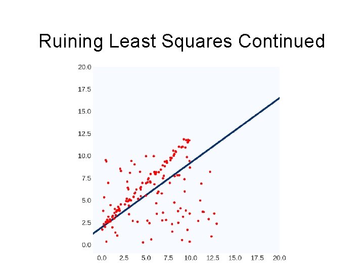
Ruining Least Squares

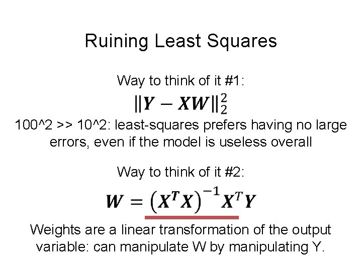
Ruining Least Squares Way to think of it #1: 100^2 >> 10^2: least-squares prefers having no large errors, even if the model is useless overall Way to think of it #2: Weights are a linear transformation of the output variable: can manipulate W by manipulating Y.

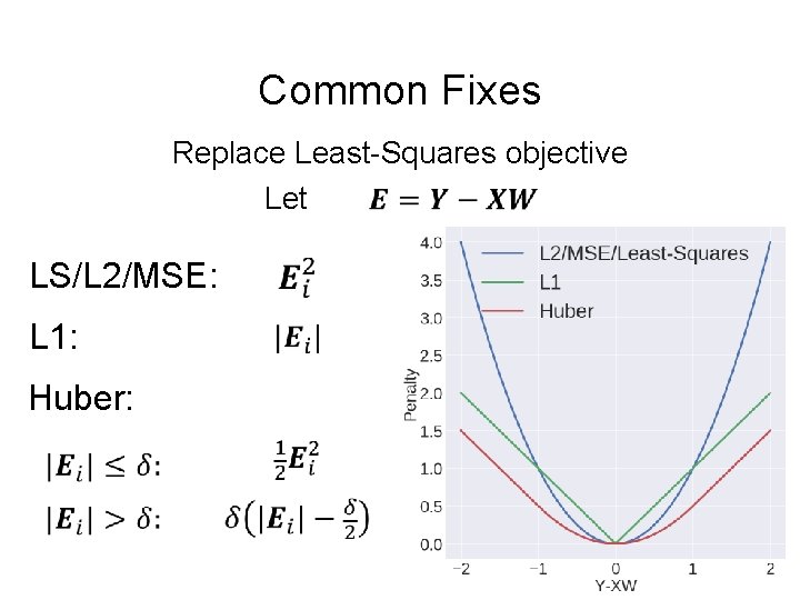
Common Fixes Replace Least-Squares objective Let LS/L 2/MSE: L 1: Huber:

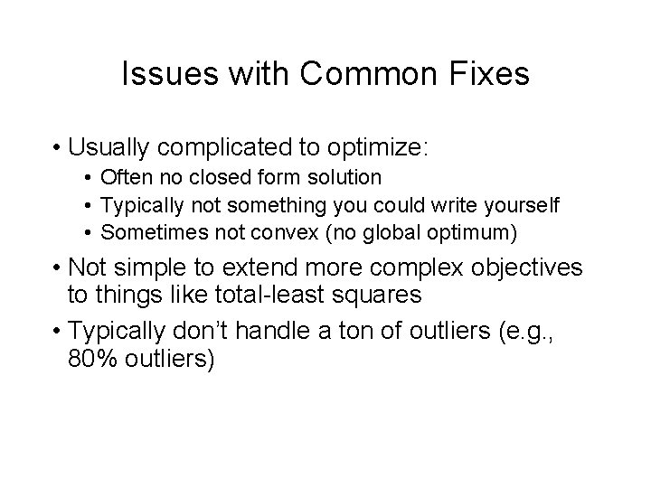
Issues with Common Fixes • Usually complicated to optimize: • Often no closed form solution • Typically not something you could write yourself • Sometimes not convex (no global optimum) • Not simple to extend more complex objectives to things like total-least squares • Typically don’t handle a ton of outliers (e. g. , 80% outliers)

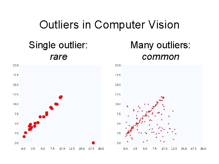
Outliers in Computer Vision Single outlier: rare Many outliers: common

Ruining Least Squares Continued

Ruining Least Squares Continued

A Simple, Yet Clever Idea • What we really want: model explains many points “well” • Least Squares: model makes as few big mistakes as possible over the entire dataset • New objective: find model for which error is “small” for as many data points as possible • Method: RANSAC (RAndom SAmple Consensus) M. A. Fischler, R. C. Bolles. Random Sample Consensus: A Paradigm for Model Fitting with Applications to Image Analysis and Automated Cartography. Comm. of the ACM, Vol 24, pp 381 -395, 1981.

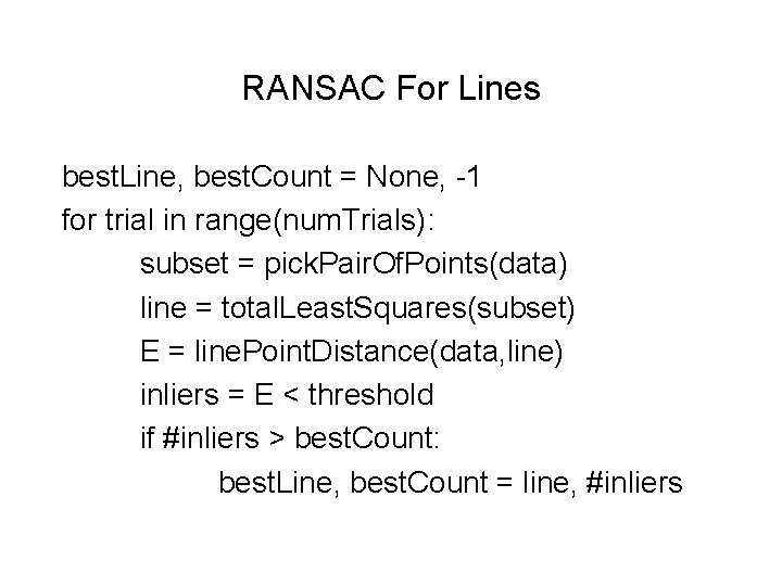
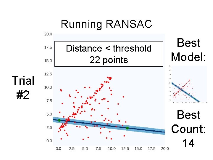
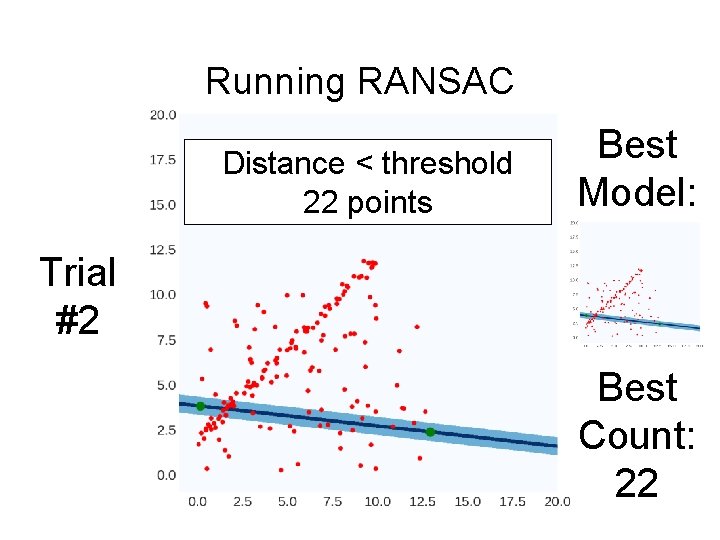
RANSAC For Lines best. Line, best. Count = None, -1 for trial in range(num. Trials): subset = pick. Pair. Of. Points(data) line = total. Least. Squares(subset) E = line. Point. Distance(data, line) inliers = E < threshold if #inliers > best. Count: best. Line, best. Count = line, #inliers

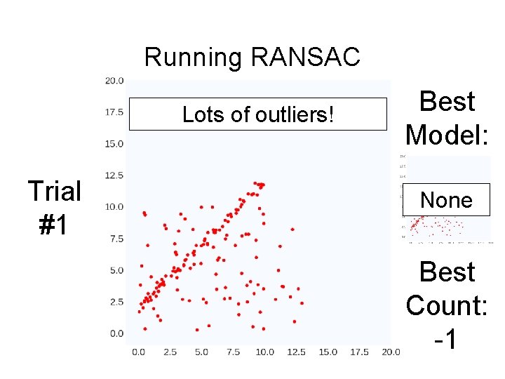
Running RANSAC Lots of outliers! Trial #1 Best Model: None Best Count: -1

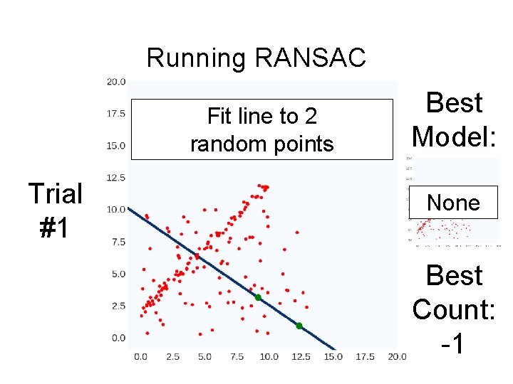
Running RANSAC Fit line to 2 random points Trial #1 Best Model: None Best Count: -1
![Running RANSAC Pointline distance n Tx y d Trial 1 Best Model None Running RANSAC Point/line distance |n. T[x, y] – d| Trial #1 Best Model: None](https://slidetodoc.com/presentation_image_h2/ad1127fd351aeefe2384aeae6fc2a870/image-37.jpg)
Running RANSAC Point/line distance |n. T[x, y] – d| Trial #1 Best Model: None Best Count: -1

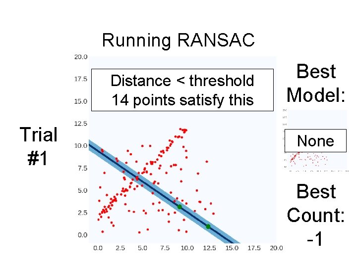
Running RANSAC Distance < threshold 14 points satisfy this Trial #1 Best Model: None Best Count: -1

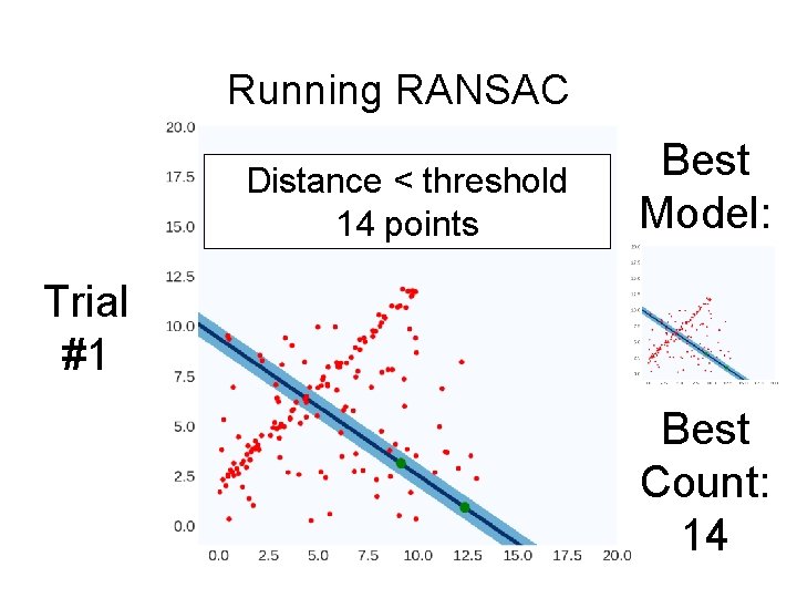
Running RANSAC Distance < threshold 14 points Best Model: Trial #1 Best Count: 14

Running RANSAC Distance < threshold 22 points Best Model: Trial #2 Best Count: 14

Running RANSAC Distance < threshold 22 points Best Model: Trial #2 Best Count: 22

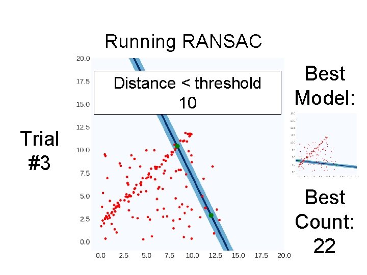
Running RANSAC Distance < threshold 10 Best Model: Trial #3 Best Count: 22

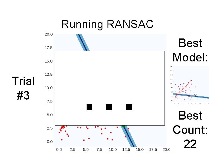
Running RANSAC Trial #3 … Best Model: Best Count: 22

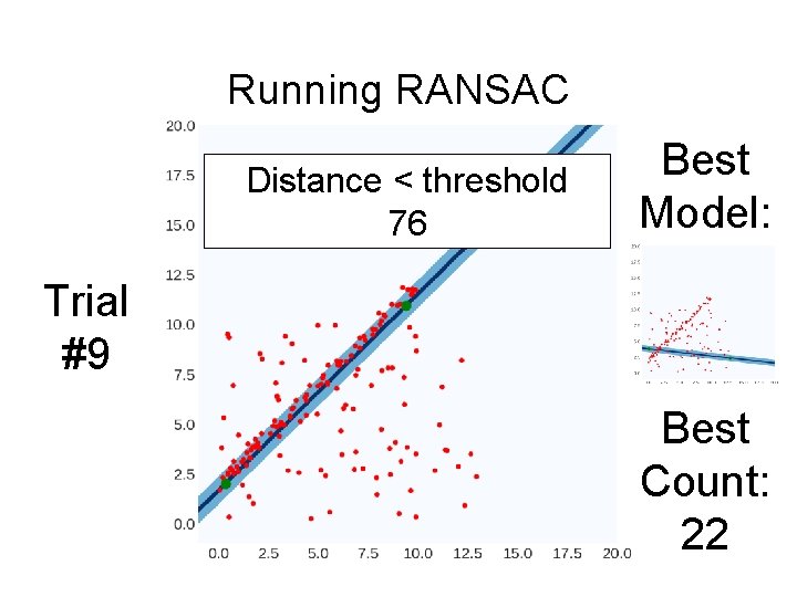
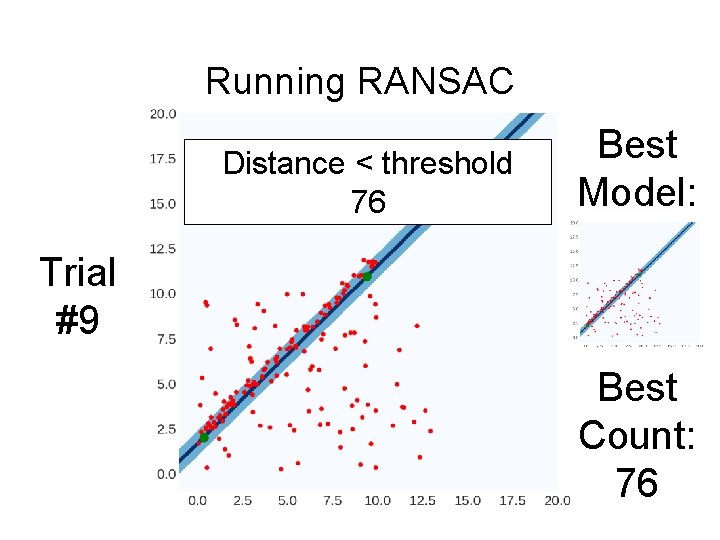
Running RANSAC Distance < threshold 76 Best Model: Trial #9 Best Count: 22

Running RANSAC Distance < threshold 76 Best Model: Trial #9 Best Count: 76

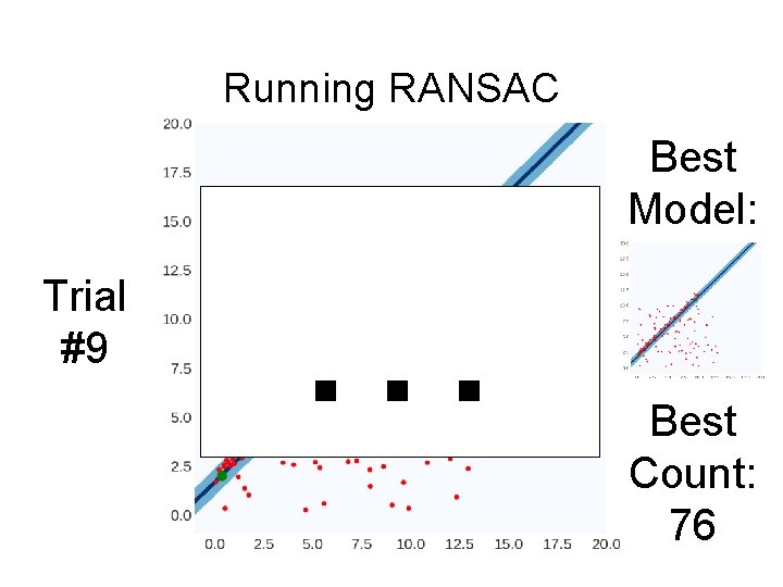
Running RANSAC Trial #9 … Best Model: Best Count: 76

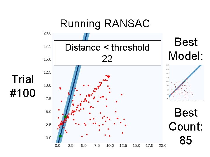
Running RANSAC Distance < threshold 22 Best Model: Trial #100 Best Count: 85

Running RANSAC Final Output of RANSAC: Best Model

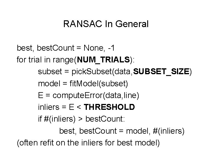
RANSAC In General best, best. Count = None, -1 for trial in range(NUM_TRIALS): subset = pick. Subset(data, SUBSET_SIZE) model = fit. Model(subset) E = compute. Error(data, line) inliers = E < THRESHOLD if #(inliers) > best. Count: best, best. Count = model, #(inliers) (often refit on the inliers for best model)

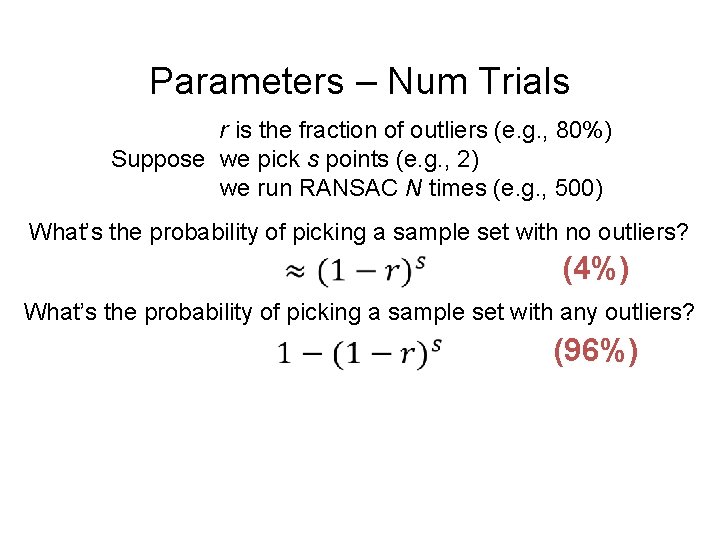
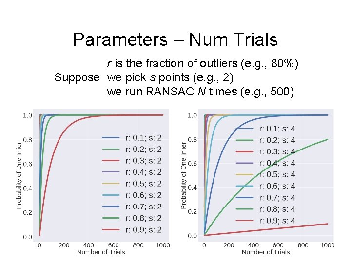
Parameters – Num Trials r is the fraction of outliers (e. g. , 80%) Suppose we pick s points (e. g. , 2) we run RANSAC N times (e. g. , 500) What’s the probability of picking a sample set with no outliers? (4%) What’s the probability of picking a sample set with any outliers? (96%)

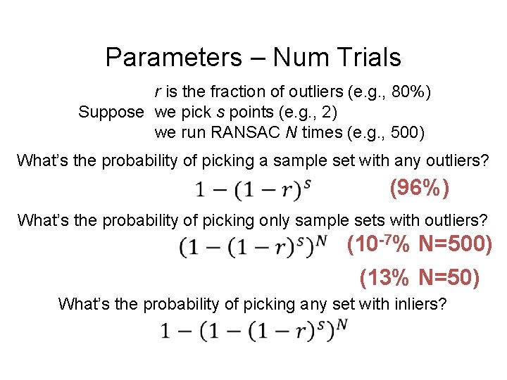
Parameters – Num Trials r is the fraction of outliers (e. g. , 80%) Suppose we pick s points (e. g. , 2) we run RANSAC N times (e. g. , 500) What’s the probability of picking a sample set with any outliers? (96%) What’s the probability of picking only sample sets with outliers? (10 -7% N=500) (13% N=50) What’s the probability of picking any set with inliers?

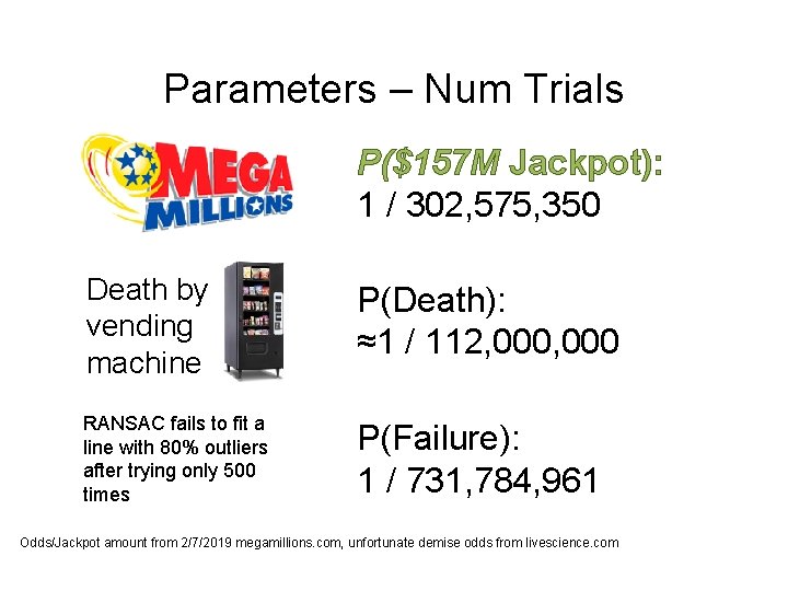
Parameters – Num Trials P($157 M Jackpot): 1 / 302, 575, 350 Death by vending machine P(Death): ≈1 / 112, 000 RANSAC fails to fit a line with 80% outliers after trying only 500 times P(Failure): 1 / 731, 784, 961 Odds/Jackpot amount from 2/7/2019 megamillions. com, unfortunate demise odds from livescience. com

Parameters – Num Trials r is the fraction of outliers (e. g. , 80%) Suppose we pick s points (e. g. , 2) we run RANSAC N times (e. g. , 500)

Parameters – Subset Size • Always the smallest possible set for fitting the model. • Minimum number for lines: 2 data points • Minimum number of planes: how many? • Why intuitively? • You’ll find out more precisely in homework 3.

Parameters – Threshold • Common sense; there’s no magical threshold

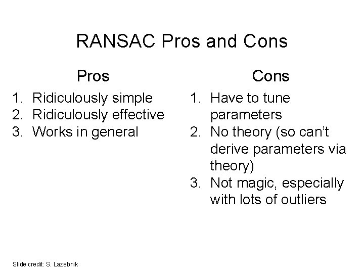
RANSAC Pros and Cons Pros 1. Ridiculously simple 2. Ridiculously effective 3. Works in general Slide credit: S. Lazebnik Cons 1. Have to tune parameters 2. No theory (so can’t derive parameters via theory) 3. Not magic, especially with lots of outliers

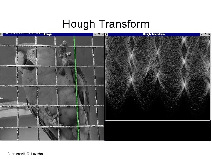
Hough Transform Slide credit: S. Lazebnik

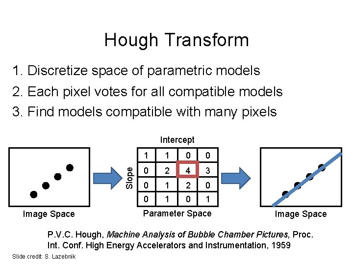
Hough Transform 1. Discretize space of parametric models 2. Each pixel votes for all compatible models 3. Find models compatible with many pixels Slope Intercept Image Space 1 1 0 0 0 2 4 3 0 1 2 0 0 1 Parameter Space Image Space P. V. C. Hough, Machine Analysis of Bubble Chamber Pictures, Proc. Int. Conf. High Energy Accelerators and Instrumentation, 1959 Slide credit: S. Lazebnik

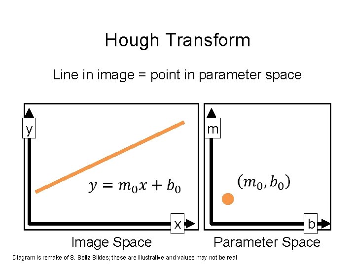
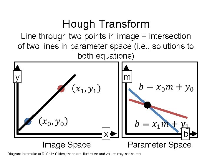
Hough Transform Line in image = point in parameter space m y x Image Space b Parameter Space Diagram is remake of S. Seitz Slides; these are illustrative and values may not be real

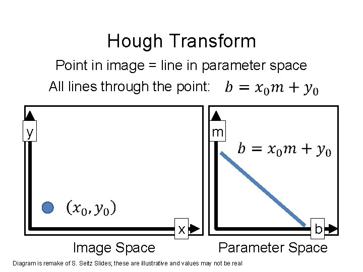
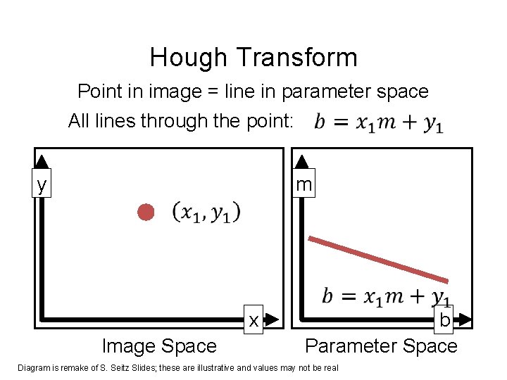
Hough Transform Point in image = line in parameter space All lines through the point: m y x Image Space b Parameter Space Diagram is remake of S. Seitz Slides; these are illustrative and values may not be real

Hough Transform Point in image = line in parameter space All lines through the point: m y x Image Space b Parameter Space Diagram is remake of S. Seitz Slides; these are illustrative and values may not be real

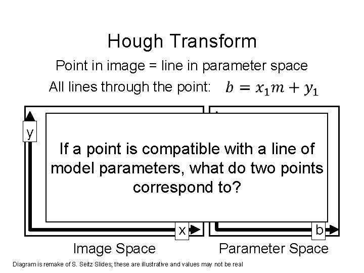
Hough Transform Point in image = line in parameter space All lines through the point: y m If a point is compatible with a line of model parameters, what do two points correspond to? x Image Space b Parameter Space Diagram is remake of S. Seitz Slides; these are illustrative and values may not be real

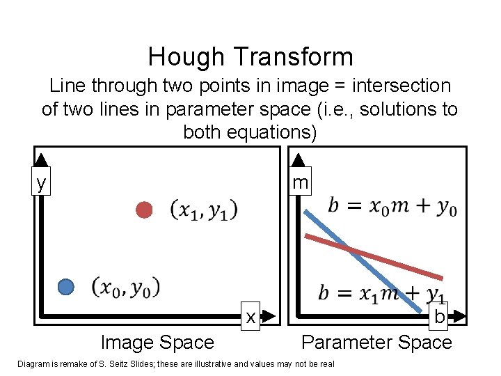
Hough Transform Line through two points in image = intersection of two lines in parameter space (i. e. , solutions to both equations) m y x Image Space b Parameter Space Diagram is remake of S. Seitz Slides; these are illustrative and values may not be real

Hough Transform Line through two points in image = intersection of two lines in parameter space (i. e. , solutions to both equations) m y x Image Space b Parameter Space Diagram is remake of S. Seitz Slides; these are illustrative and values may not be real

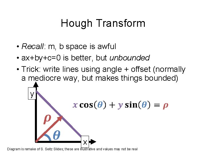
Hough Transform • Recall: m, b space is awful • ax+by+c=0 is better, but unbounded • Trick: write lines using angle + offset (normally a mediocre way, but makes things bounded) y x Diagram is remake of S. Seitz Slides; these are illustrative and values may not be real

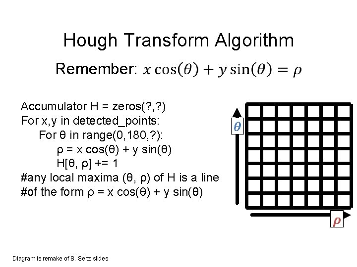
Hough Transform Algorithm Remember: Accumulator H = zeros(? , ? ) For x, y in detected_points: For θ in range(0, 180, ? ): ρ = x cos(θ) + y sin(θ) H[θ, ρ] += 1 #any local maxima (θ, ρ) of H is a line #of the form ρ = x cos(θ) + y sin(θ) Diagram is remake of S. Seitz slides

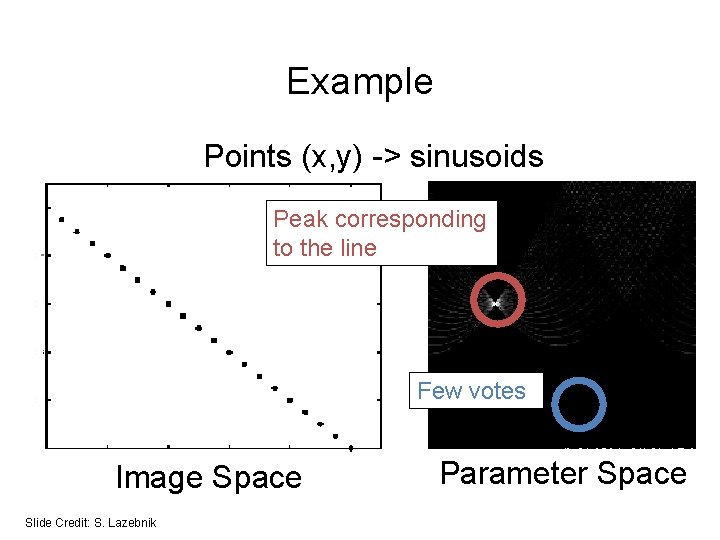
Example Points (x, y) -> sinusoids Peak corresponding to the line Few votes Image Space Slide Credit: S. Lazebnik Parameter Space

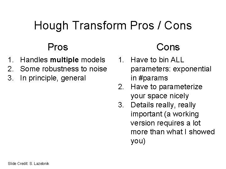
Hough Transform Pros / Cons Pros Cons 1. Handles multiple models 2. Some robustness to noise 3. In principle, general 1. Have to bin ALL parameters: exponential in #params 2. Have to parameterize your space nicely 3. Details really, really important (a working version requires a lot more than what I showed you) Slide Credit: S. Lazebnik

Next Time • What happens with fitting more complex transformations?