Scales and Descriptors EECS 442 David Fouhey Fall

Scales and Descriptors EECS 442 – David Fouhey Fall 2019, University of Michigan http: //web. eecs. umich. edu/~fouhey/teaching/EECS 442_F 19/

Administrivia • HW 1 due tonight (modulo late days) • HW 2 out tonight • Collaborate • Read the syllabus for what’s allowed

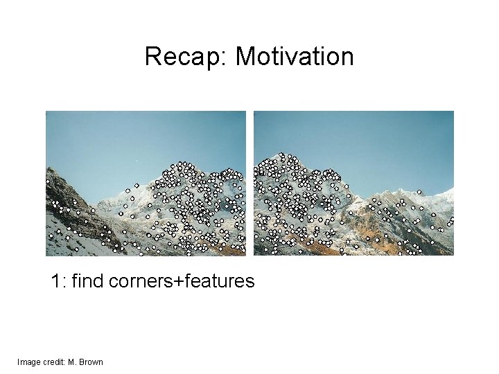
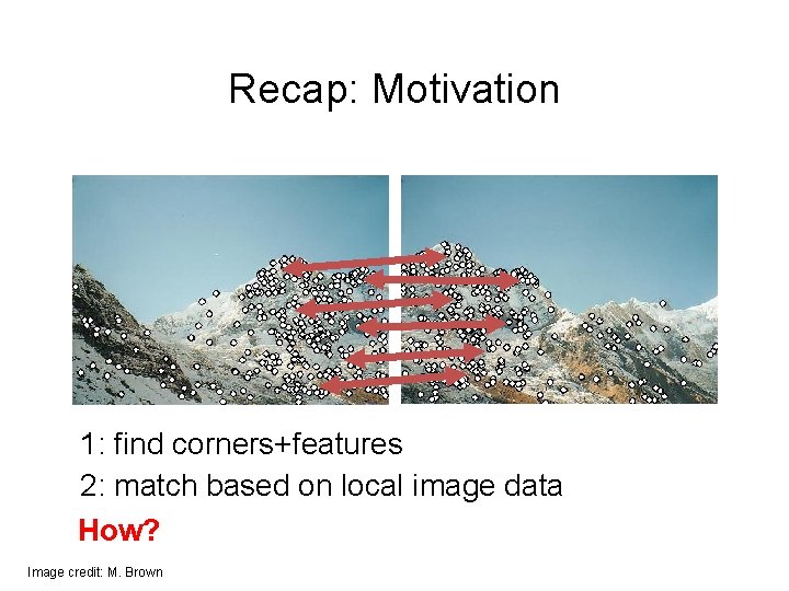
Recap: Motivation 1: find corners+features Image credit: M. Brown

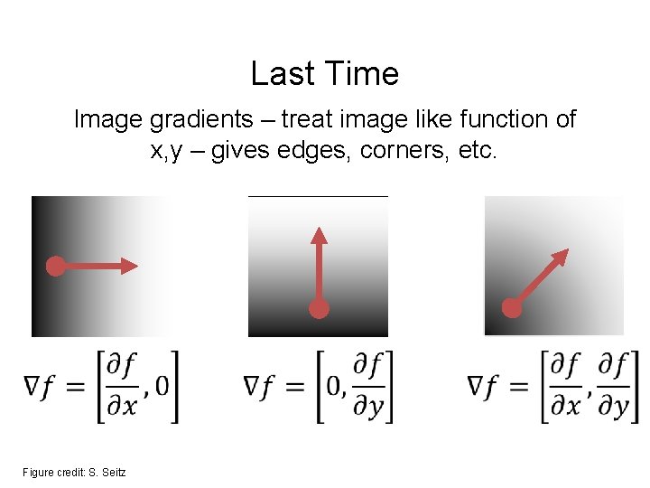
Last Time Image gradients – treat image like function of x, y – gives edges, corners, etc. Figure credit: S. Seitz

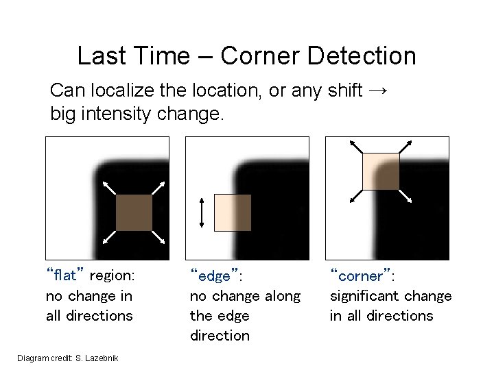
Last Time – Corner Detection Can localize the location, or any shift → big intensity change. “flat” region: no change in all directions Diagram credit: S. Lazebnik “edge”: no change along the edge direction “corner”: significant change in all directions

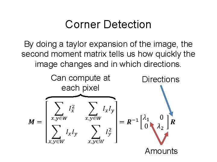
Corner Detection By doing a taylor expansion of the image, the second moment matrix tells us how quickly the image changes and in which directions. Can compute at each pixel Directions Amounts

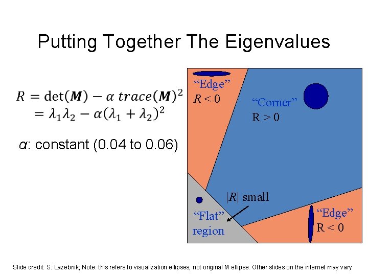
Putting Together The Eigenvalues “Edge” R<0 “Corner” R>0 α: constant (0. 04 to 0. 06) |R| small “Flat” region “Edge” R<0 Slide credit: S. Lazebnik; Note: this refers to visualization ellipses, not original M ellipse. Other slides on the internet may vary

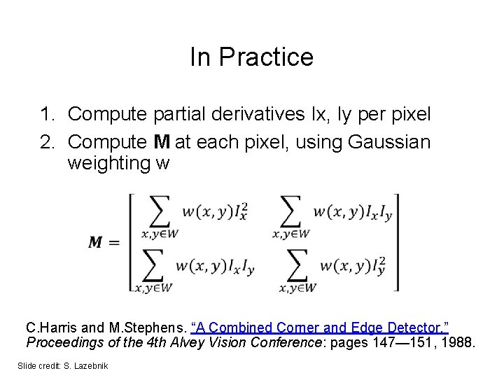
In Practice 1. Compute partial derivatives Ix, Iy per pixel 2. Compute M at each pixel, using Gaussian weighting w C. Harris and M. Stephens. “A Combined Corner and Edge Detector. ” Proceedings of the 4 th Alvey Vision Conference: pages 147— 151, 1988. Slide credit: S. Lazebnik

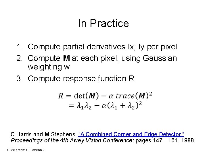
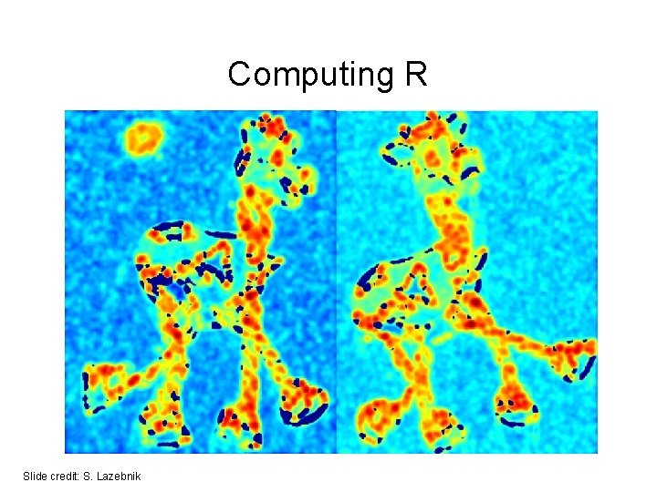
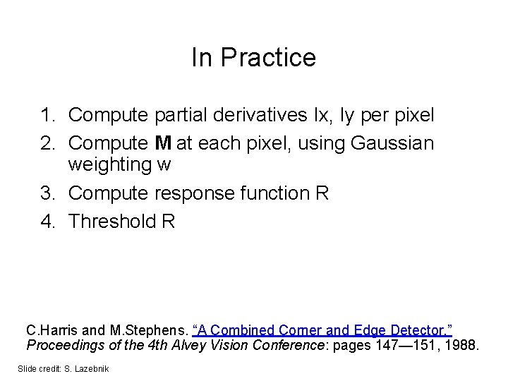
In Practice 1. Compute partial derivatives Ix, Iy per pixel 2. Compute M at each pixel, using Gaussian weighting w 3. Compute response function R C. Harris and M. Stephens. “A Combined Corner and Edge Detector. ” Proceedings of the 4 th Alvey Vision Conference: pages 147— 151, 1988. Slide credit: S. Lazebnik

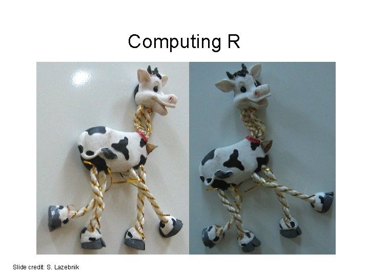
Computing R Slide credit: S. Lazebnik

Computing R Slide credit: S. Lazebnik

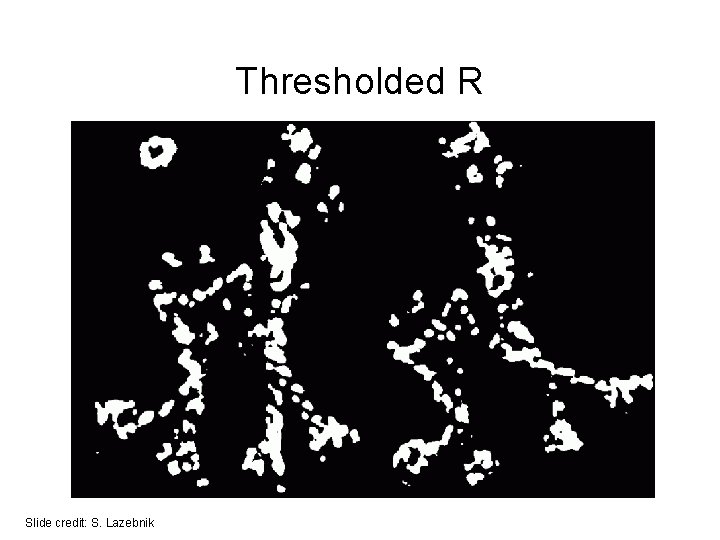
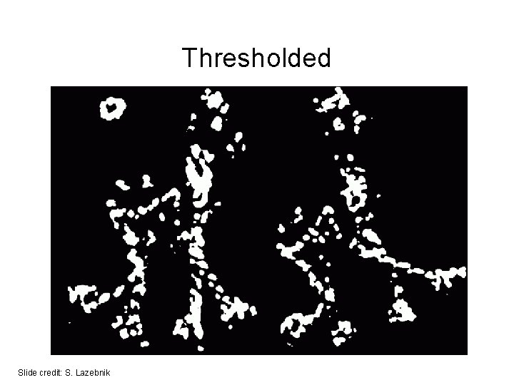
In Practice 1. Compute partial derivatives Ix, Iy per pixel 2. Compute M at each pixel, using Gaussian weighting w 3. Compute response function R 4. Threshold R C. Harris and M. Stephens. “A Combined Corner and Edge Detector. ” Proceedings of the 4 th Alvey Vision Conference: pages 147— 151, 1988. Slide credit: S. Lazebnik

Thresholded R Slide credit: S. Lazebnik

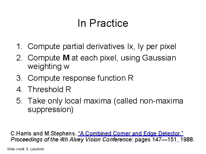
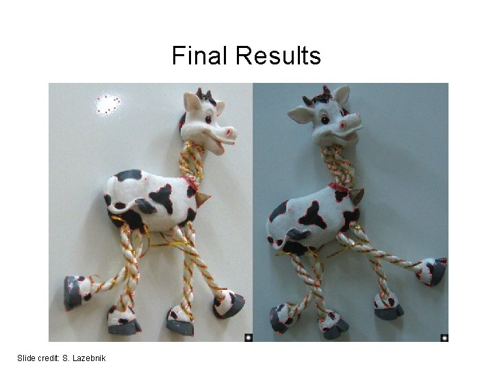
In Practice 1. Compute partial derivatives Ix, Iy per pixel 2. Compute M at each pixel, using Gaussian weighting w 3. Compute response function R 4. Threshold R 5. Take only local maxima (called non-maxima suppression) C. Harris and M. Stephens. “A Combined Corner and Edge Detector. ” Proceedings of the 4 th Alvey Vision Conference: pages 147— 151, 1988. Slide credit: S. Lazebnik

Thresholded Slide credit: S. Lazebnik

Final Results Slide credit: S. Lazebnik

Desirable Properties If our detectors are repeatable, they should be: • Invariant to some things: image is transformed and corners remain the same • Covariant/equivariant with some things: image is transformed and corners transform with it. Slide credit: S. Lazebnik

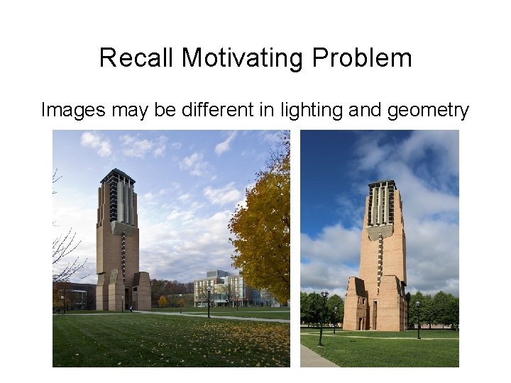
Recall Motivating Problem Images may be different in lighting and geometry

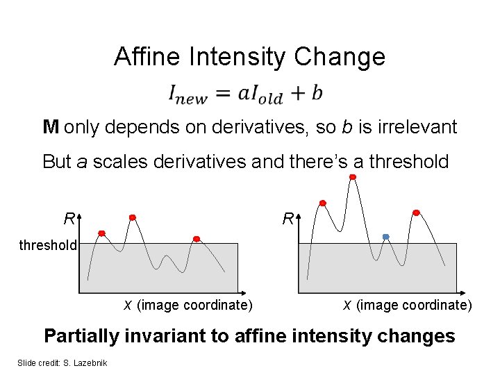
Affine Intensity Change M only depends on derivatives, so b is irrelevant But a scales derivatives and there’s a threshold R R threshold x (image coordinate) Partially invariant to affine intensity changes Slide credit: S. Lazebnik

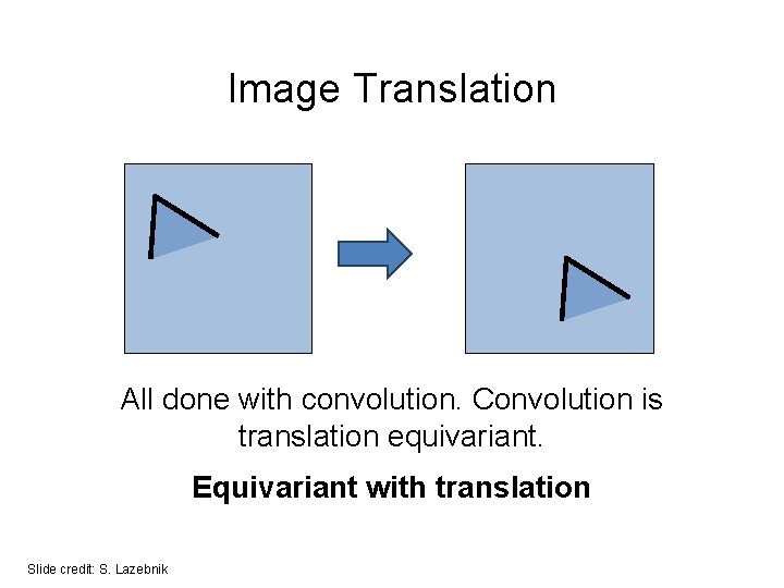
Image Translation All done with convolution. Convolution is translation equivariant. Equivariant with translation Slide credit: S. Lazebnik

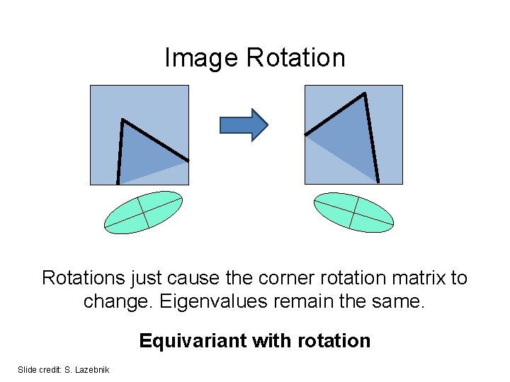
Image Rotations just cause the corner rotation matrix to change. Eigenvalues remain the same. Equivariant with rotation Slide credit: S. Lazebnik

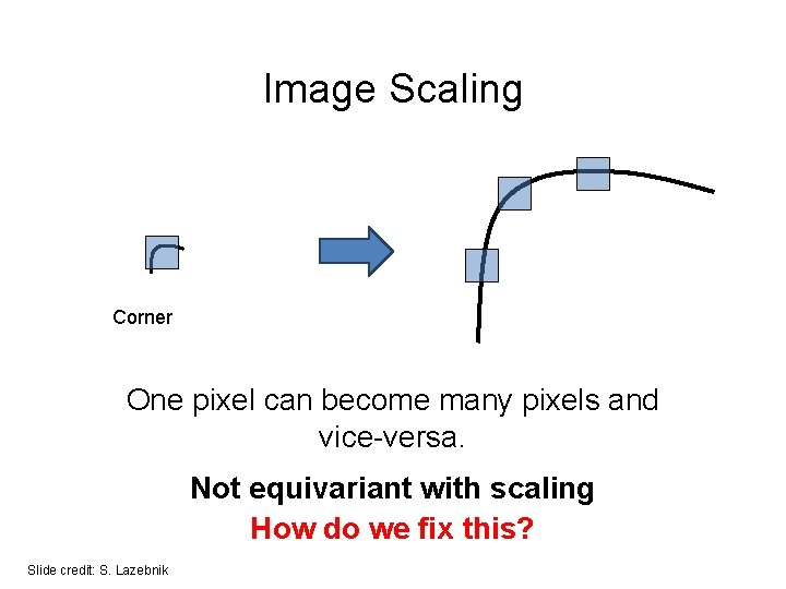
Image Scaling Corner One pixel can become many pixels and vice-versa. Not equivariant with scaling How do we fix this? Slide credit: S. Lazebnik

Recap: Motivation 1: find corners+features 2: match based on local image data How? Image credit: M. Brown

Today • Fixing scaling by making detectors in both location and scale • Enabling matching between features by describing regions

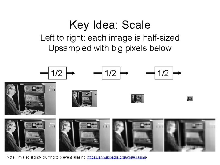
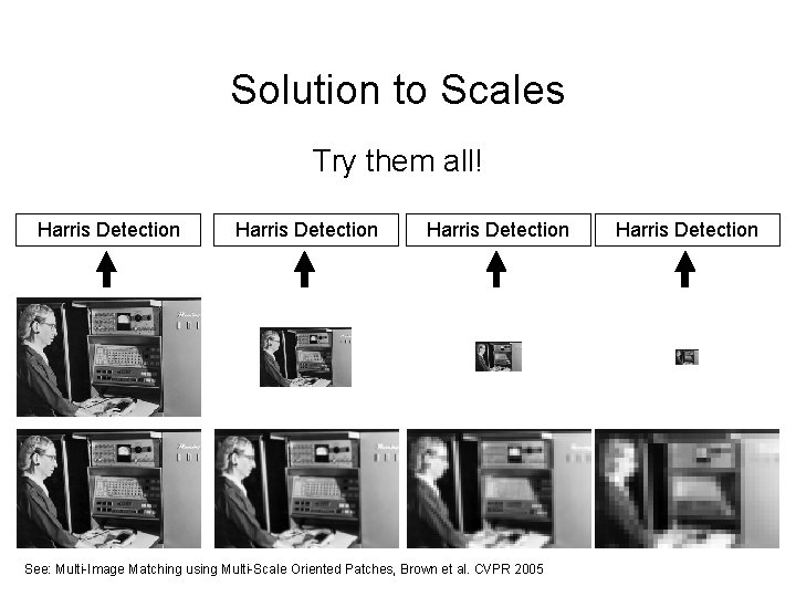
Key Idea: Scale Left to right: each image is half-sized Upsampled with big pixels below 1/2 Note: I’m also slightly blurring to prevent aliasing (https: //en. wikipedia. org/wiki/Aliasing) 1/2

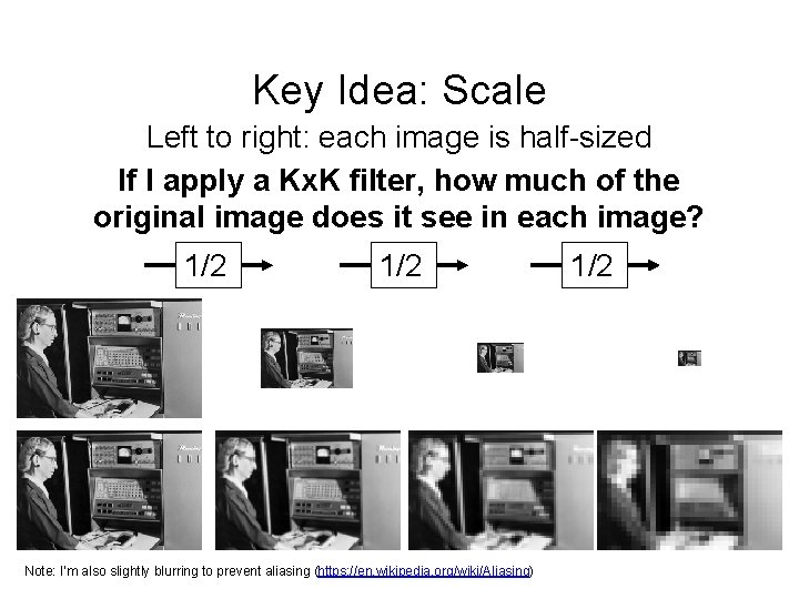
Key Idea: Scale Left to right: each image is half-sized If I apply a Kx. K filter, how much of the original image does it see in each image? 1/2 Note: I’m also slightly blurring to prevent aliasing (https: //en. wikipedia. org/wiki/Aliasing) 1/2

Solution to Scales Try them all! Harris Detection See: Multi-Image Matching using Multi-Scale Oriented Patches, Brown et al. CVPR 2005 Harris Detection

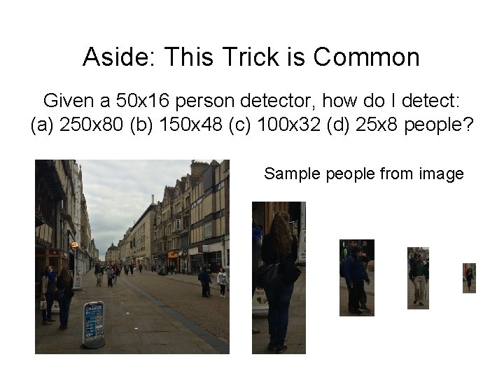
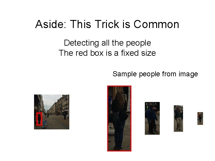
Aside: This Trick is Common Given a 50 x 16 person detector, how do I detect: (a) 250 x 80 (b) 150 x 48 (c) 100 x 32 (d) 25 x 8 people? Sample people from image

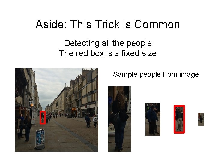
Aside: This Trick is Common Detecting all the people The red box is a fixed size Sample people from image

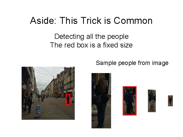
Aside: This Trick is Common Detecting all the people The red box is a fixed size Sample people from image

Aside: This Trick is Common Detecting all the people The red box is a fixed size Sample people from image

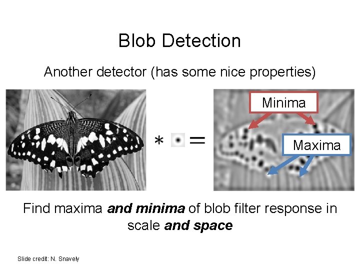
Blob Detection Another detector (has some nice properties) Minima Maxima Find maxima and minima of blob filter response in scale and space Slide credit: N. Snavely

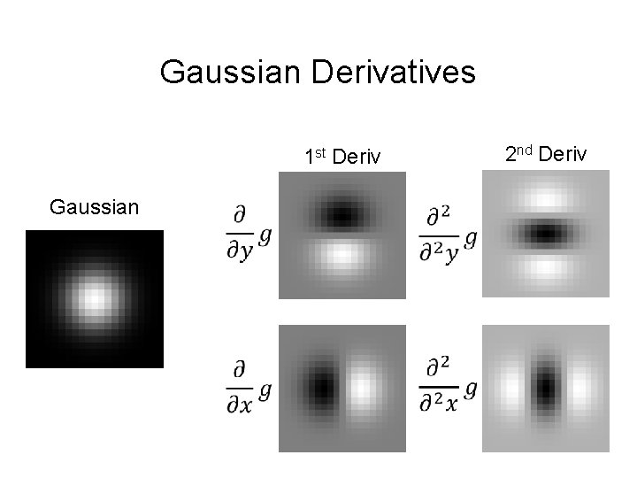
Gaussian Derivatives 2 nd Deriv 1 st Deriv Gaussian

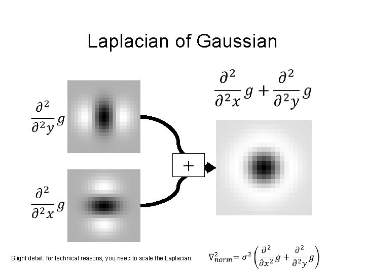
Laplacian of Gaussian + Slight detail: for technical reasons, you need to scale the Laplacian.

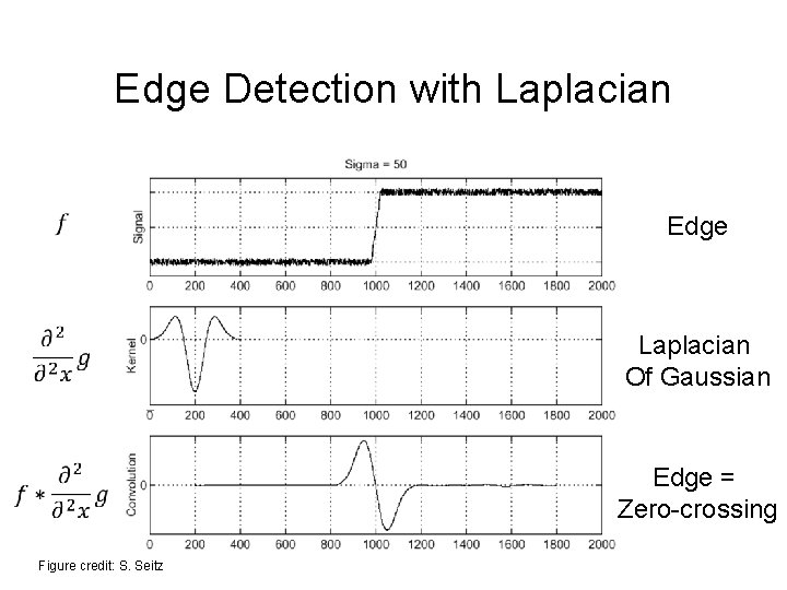
Edge Detection with Laplacian Edge Laplacian Of Gaussian Edge = Zero-crossing Figure credit: S. Seitz

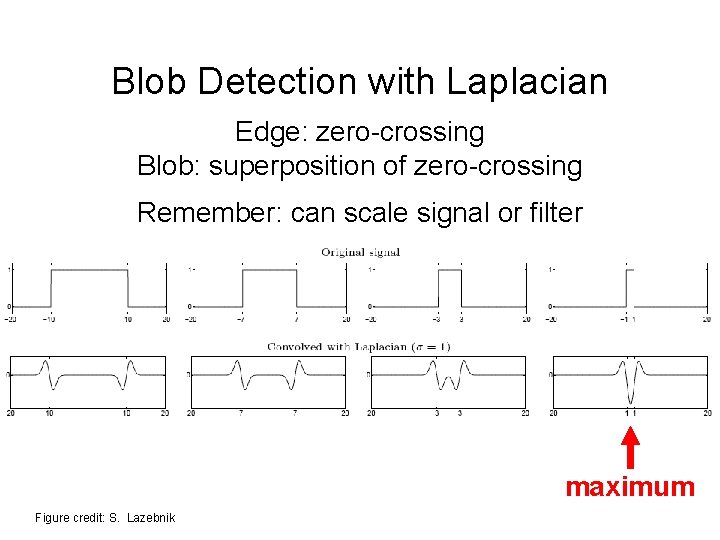
Blob Detection with Laplacian Edge: zero-crossing Blob: superposition of zero-crossing Remember: can scale signal or filter maximum Figure credit: S. Lazebnik

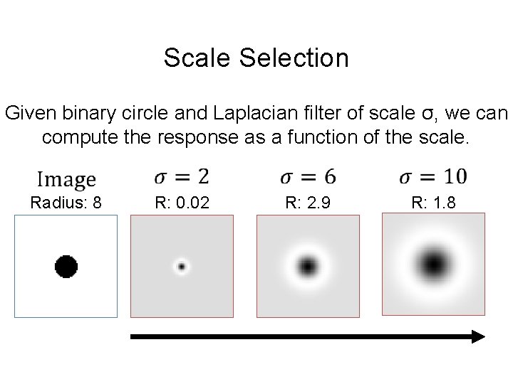
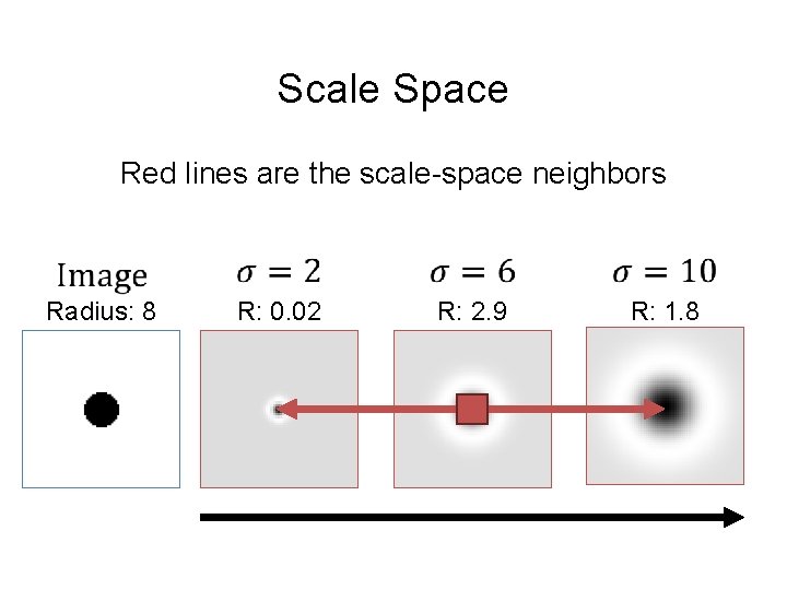
Scale Selection Given binary circle and Laplacian filter of scale σ, we can compute the response as a function of the scale. Radius: 8 R: 0. 02 R: 2. 9 R: 1. 8

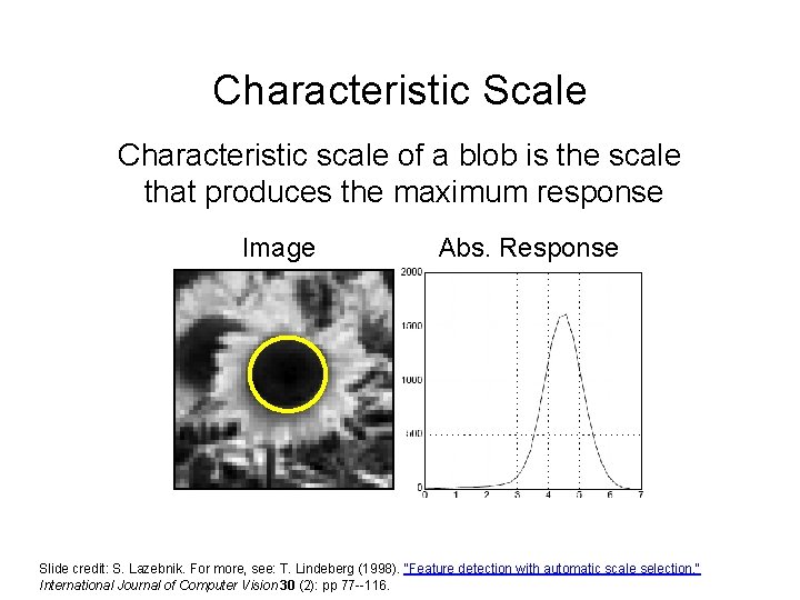
Characteristic Scale Characteristic scale of a blob is the scale that produces the maximum response Image Abs. Response Slide credit: S. Lazebnik. For more, see: T. Lindeberg (1998). "Feature detection with automatic scale selection. " International Journal of Computer Vision 30 (2): pp 77 --116.

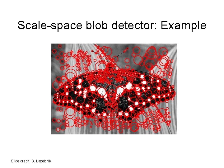
Scale-space blob detector 1. Convolve image with scale-normalized Laplacian at several scales Slide credit: S. Lazebnik

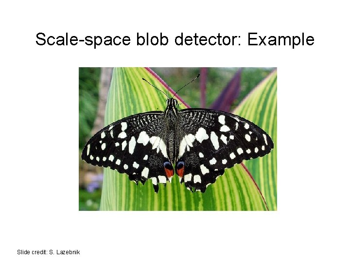
Scale-space blob detector: Example Slide credit: S. Lazebnik

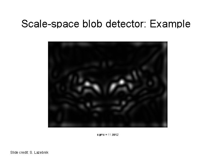
Scale-space blob detector: Example Slide credit: S. Lazebnik

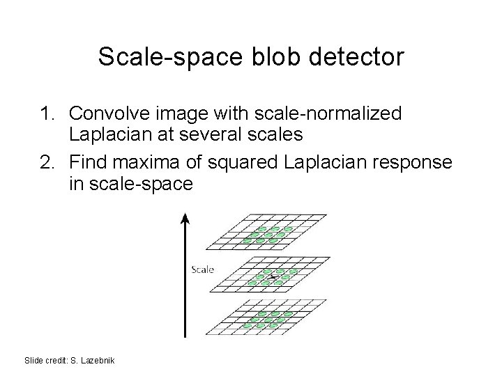
Scale-space blob detector 1. Convolve image with scale-normalized Laplacian at several scales 2. Find maxima of squared Laplacian response in scale-space Slide credit: S. Lazebnik

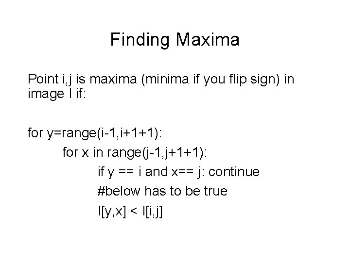
Finding Maxima Point i, j is maxima (minima if you flip sign) in image I if: for y=range(i-1, i+1+1): for x in range(j-1, j+1+1): if y == i and x== j: continue #below has to be true I[y, x] < I[i, j]

Scale Space Red lines are the scale-space neighbors Radius: 8 R: 0. 02 R: 2. 9 R: 1. 8

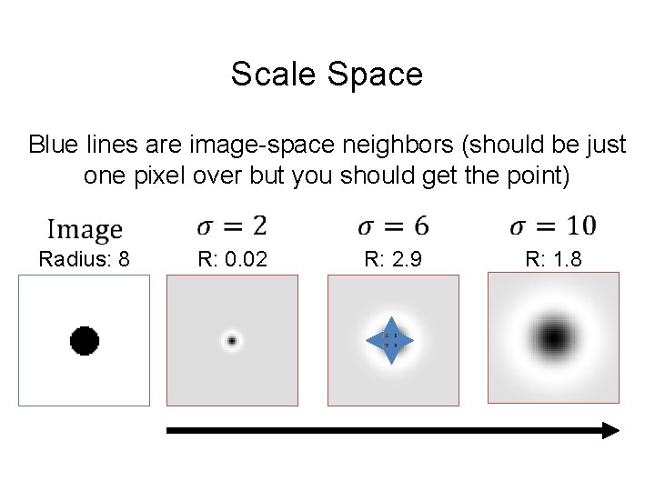
Scale Space Blue lines are image-space neighbors (should be just one pixel over but you should get the point) Radius: 8 R: 0. 02 R: 2. 9 R: 1. 8

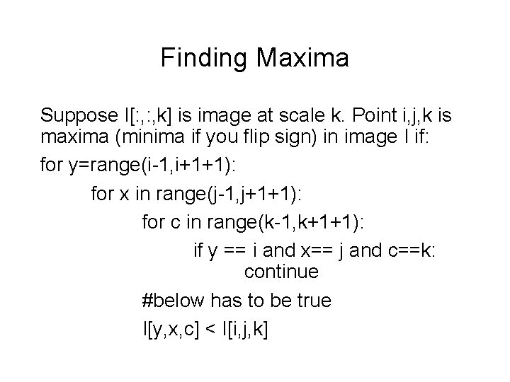
Finding Maxima Suppose I[: , k] is image at scale k. Point i, j, k is maxima (minima if you flip sign) in image I if: for y=range(i-1, i+1+1): for x in range(j-1, j+1+1): for c in range(k-1, k+1+1): if y == i and x== j and c==k: continue #below has to be true I[y, x, c] < I[i, j, k]

Scale-space blob detector: Example Slide credit: S. Lazebnik

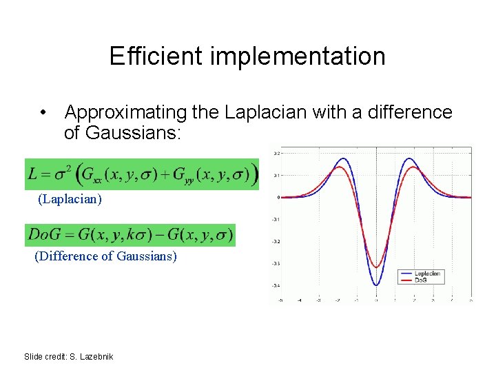
Efficient implementation • Approximating the Laplacian with a difference of Gaussians: (Laplacian) (Difference of Gaussians) Slide credit: S. Lazebnik

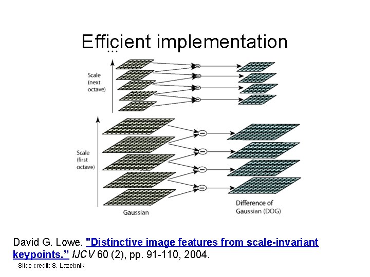
Efficient implementation David G. Lowe. "Distinctive image features from scale-invariant keypoints. ” IJCV 60 (2), pp. 91 -110, 2004. Slide credit: S. Lazebnik

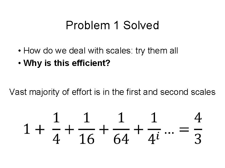
Problem 1 Solved • How do we deal with scales: try them all • Why is this efficient? Vast majority of effort is in the first and second scales

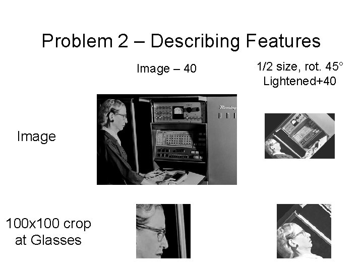
Problem 2 – Describing Features Image – 40 Image 100 x 100 crop at Glasses 1/2 size, rot. 45° Lightened+40

Problem 2 – Describing Features Once we’ve found a corner/blobs, we can’t just use the image nearby. What about: 1. Scale? 2. Rotation? 3. Additive light?

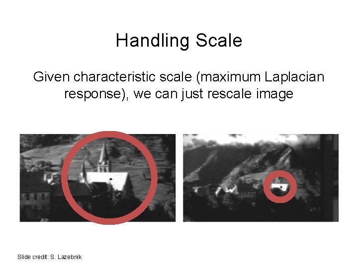
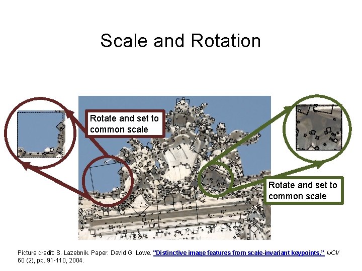
Handling Scale Given characteristic scale (maximum Laplacian response), we can just rescale image Slide credit: S. Lazebnik

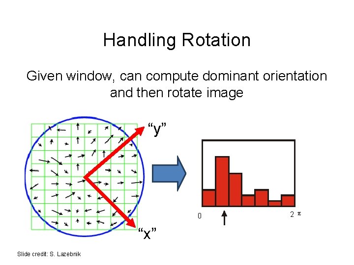
Handling Rotation Given window, can compute dominant orientation and then rotate image “y” 0 “x” Slide credit: S. Lazebnik 2 p

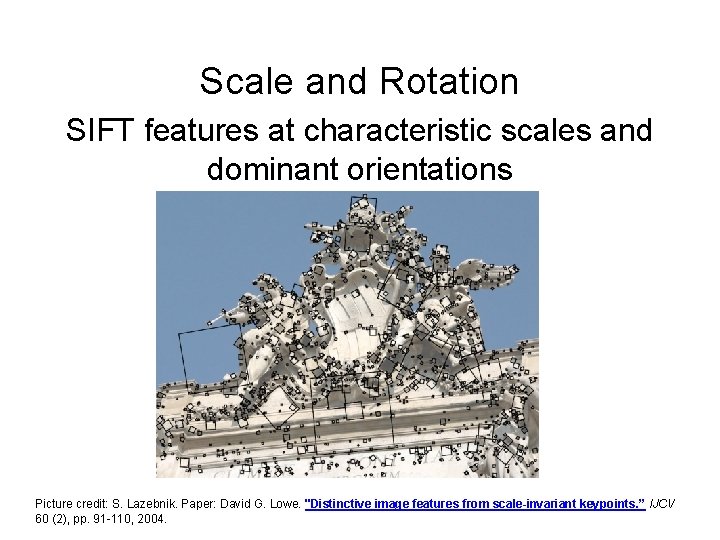
Scale and Rotation SIFT features at characteristic scales and dominant orientations Picture credit: S. Lazebnik. Paper: David G. Lowe. "Distinctive image features from scale-invariant keypoints. ” IJCV 60 (2), pp. 91 -110, 2004.

Scale and Rotation Rotate and set to common scale j Rotate and set to common scale Picture credit: S. Lazebnik. Paper: David G. Lowe. "Distinctive image features from scale-invariant keypoints. ” IJCV 60 (2), pp. 91 -110, 2004.

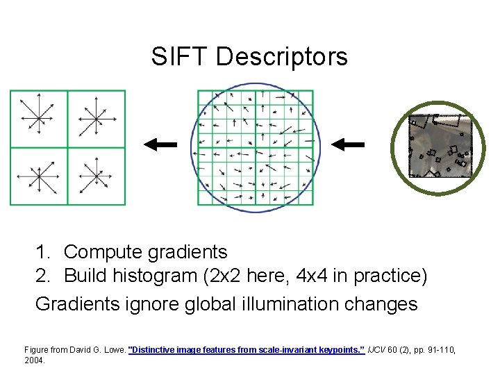
SIFT Descriptors j 1. Compute gradients 2. Build histogram (2 x 2 here, 4 x 4 in practice) Gradients ignore global illumination changes Figure from David G. Lowe. "Distinctive image features from scale-invariant keypoints. ” IJCV 60 (2), pp. 91 -110, 2004.

SIFT Descriptors • In principle: build a histogram of the gradients • In reality: quite complicated • • Gaussian weighting: smooth response Normalization: reduces illumination effects Clamping Affine adaptation

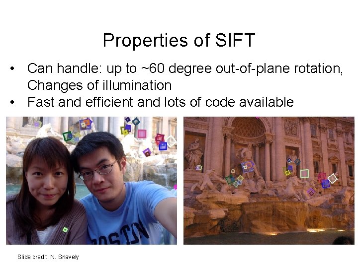
Properties of SIFT • Can handle: up to ~60 degree out-of-plane rotation, Changes of illumination • Fast and efficient and lots of code available Slide credit: N. Snavely

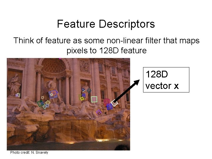
Feature Descriptors Think of feature as some non-linear filter that maps pixels to 128 D feature 128 D vector x Photo credit: N. Snavely

Using Descriptors • Instance Matching • Category recognition

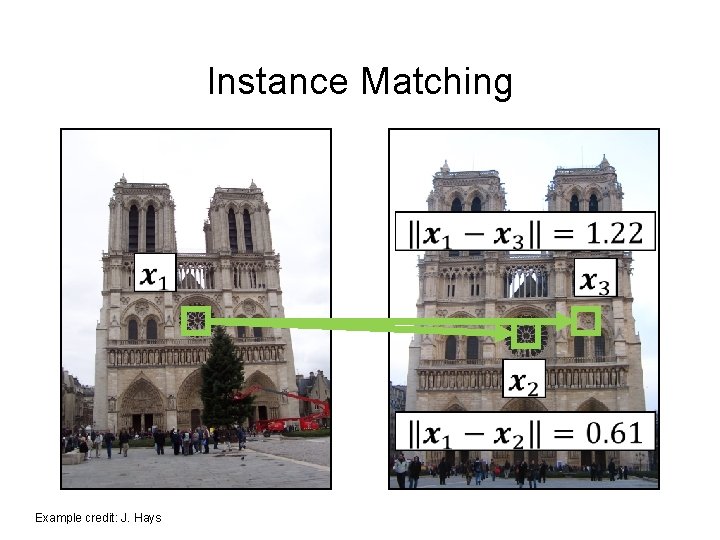
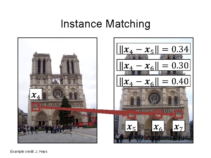
Instance Matching Example credit: J. Hays

Instance Matching Example credit: J. Hays

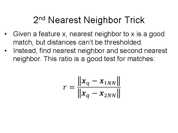
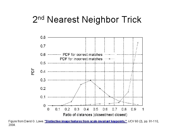
2 nd Nearest Neighbor Trick • Given a feature x, nearest neighbor to x is a good match, but distances can’t be thresholded. • Instead, find nearest neighbor and second nearest neighbor. This ratio is a good test for matches:

2 nd Nearest Neighbor Trick Figure from David G. Lowe. "Distinctive image features from scale-invariant keypoints. ” IJCV 60 (2), pp. 91 -110, 2004.

Extra Reading for the Curious

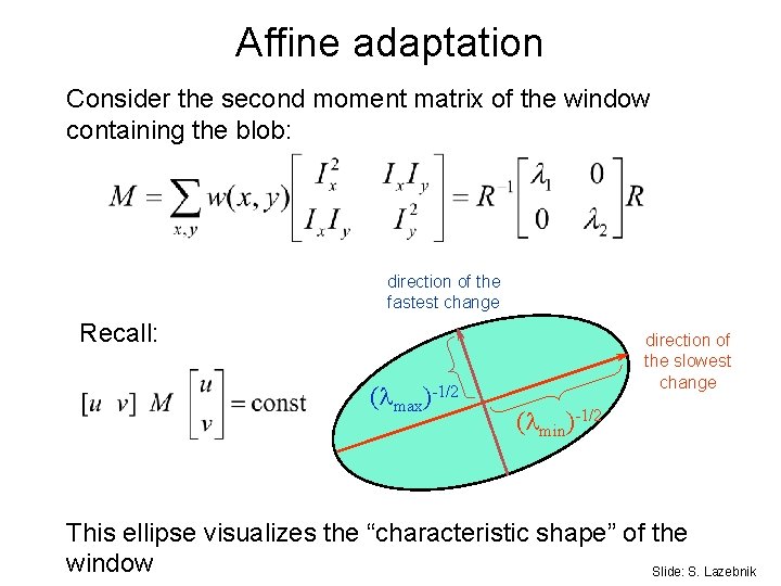
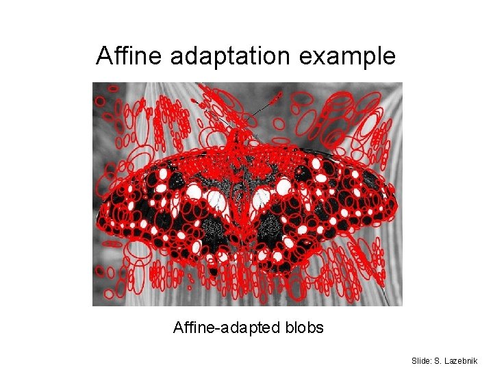
Affine adaptation Consider the second moment matrix of the window containing the blob: direction of the fastest change Recall: ( max)-1/2 direction of the slowest change ( min)-1/2 This ellipse visualizes the “characteristic shape” of the window Slide: S. Lazebnik

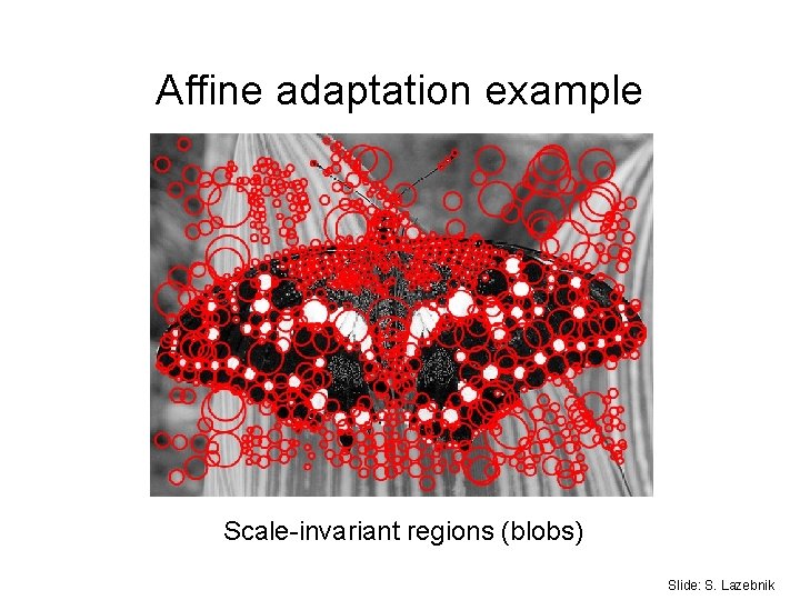
Affine adaptation example Scale-invariant regions (blobs) Slide: S. Lazebnik

Affine adaptation example Affine-adapted blobs Slide: S. Lazebnik