Text Classification Classification Learning aka supervised learning Given

Text Classification

Classification Learning (aka supervised learning) • Given labelled examples of a concept (called training examples) • Learn to predict the class label of new (unseen) examples – E. g. Given examples of fradulent and nonfradulent credit card transactions, learn to predict whether or not a new transaction is fradulent • How does it differ from Clustering?

Many uses of Text Classification • Text classification is the task of classifying text documents to multiple classes – Is this mail spam? – Is this article from comp. ai or misc. piano? – Is this article likely to be relevant to user X? – Is this page likely to lead me to pages relevant to my topic? (as in topic-specific crawling) – Is this book possibly of interest to the user?

Classification vs. Clustering • Coming from Clustering, classification seems significantly simple… • You are already given the clusters and names (over the training data) • All you need to do is to decide, for the test data, which cluster it should belong to. • Seems like a simple distance computation – Assign test data to the cluster whose centroid it is closest to – Assign test data to the cluster whose members seem to make the majority of its neighbors

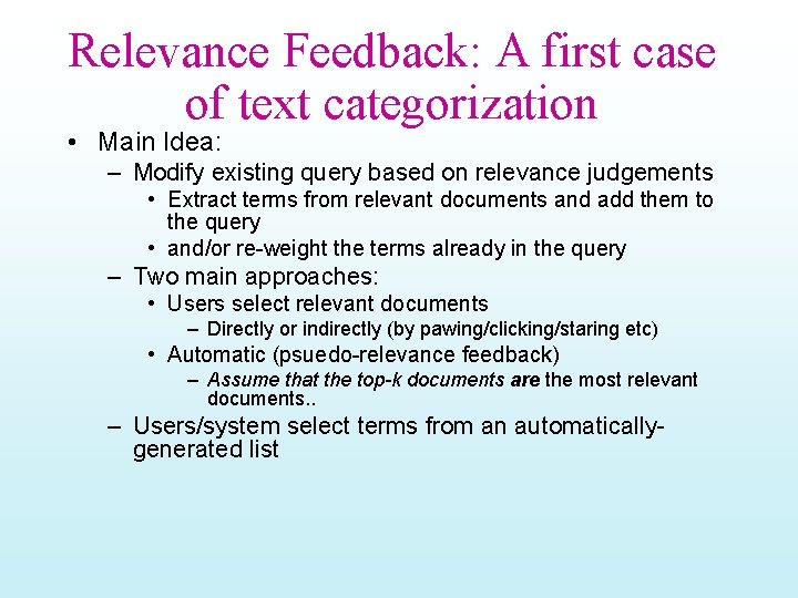
Relevance Feedback: A first case of text categorization • Main Idea: – Modify existing query based on relevance judgements • Extract terms from relevant documents and add them to the query • and/or re-weight the terms already in the query – Two main approaches: • Users select relevant documents – Directly or indirectly (by pawing/clicking/staring etc) • Automatic (psuedo-relevance feedback) – Assume that the top-k documents are the most relevant documents. . – Users/system select terms from an automaticallygenerated list

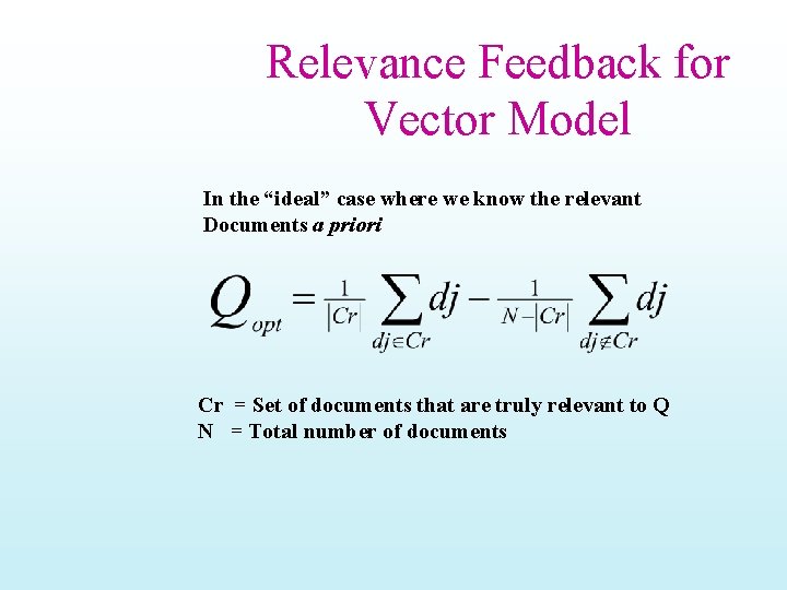
Relevance Feedback for Vector Model In the “ideal” case where we know the relevant Documents a priori Cr = Set of documents that are truly relevant to Q N = Total number of documents

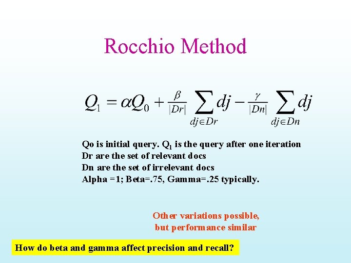
Rocchio Method Qo is initial query. Q 1 is the query after one iteration Dr are the set of relevant docs Dn are the set of irrelevant docs Alpha =1; Beta=. 75, Gamma=. 25 typically. Other variations possible, but performance similar How do beta and gamma affect precision and recall?

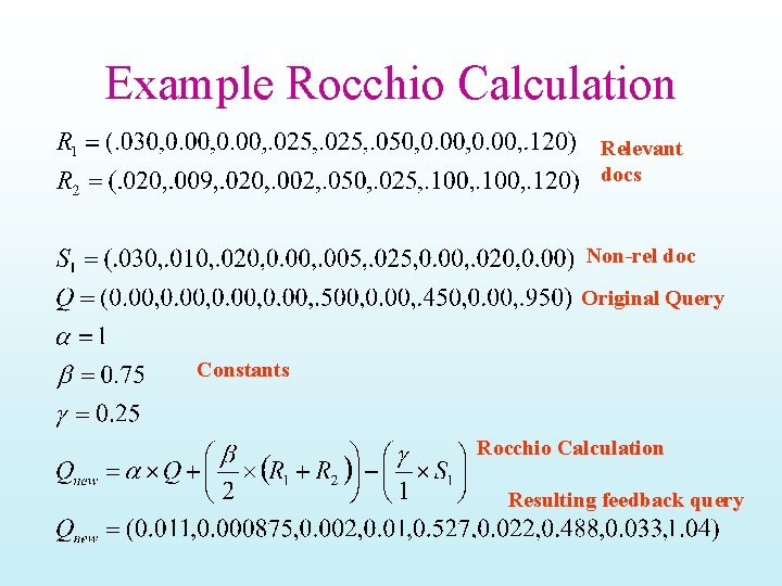
Example Rocchio Calculation Relevant docs Non-rel doc Original Query Constants Rocchio Calculation Resulting feedback query

Using Relevance Feedback • Known to improve results – in TREC-like conditions (no user involved) • What about with a user in the loop? – How might you measure this? • Precision/Recall figures for the unseen documents need to be computed

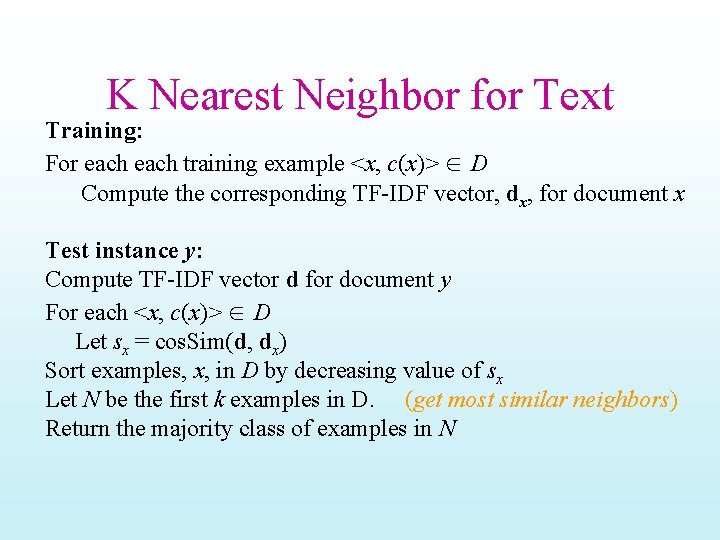
K Nearest Neighbor for Text Training: For each training example <x, c(x)> D Compute the corresponding TF-IDF vector, dx, for document x Test instance y: Compute TF-IDF vector d for document y For each <x, c(x)> D Let sx = cos. Sim(d, dx) Sort examples, x, in D by decreasing value of sx Let N be the first k examples in D. (get most similar neighbors) Return the majority class of examples in N

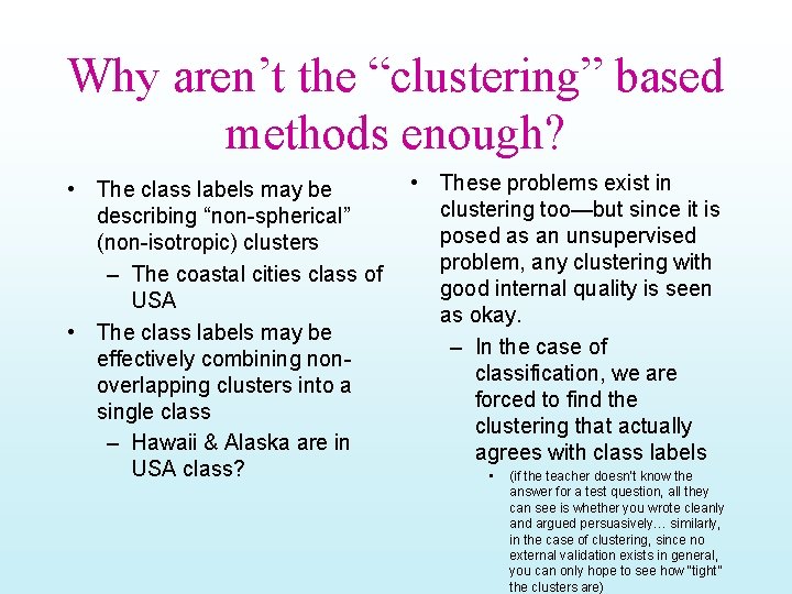
Why aren’t the “clustering” based methods enough? • The class labels may be describing “non-spherical” (non-isotropic) clusters – The coastal cities class of USA • The class labels may be effectively combining nonoverlapping clusters into a single class – Hawaii & Alaska are in USA class? • These problems exist in clustering too—but since it is posed as an unsupervised problem, any clustering with good internal quality is seen as okay. – In the case of classification, we are forced to find the clustering that actually agrees with class labels • (if the teacher doesn’t know the answer for a test question, all they can see is whether you wrote cleanly and argued persuasively… similarly, in the case of clustering, since no external validation exists in general, you can only hope to see how “tight” the clusters are)

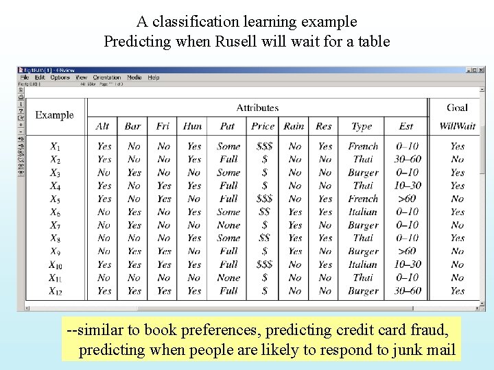
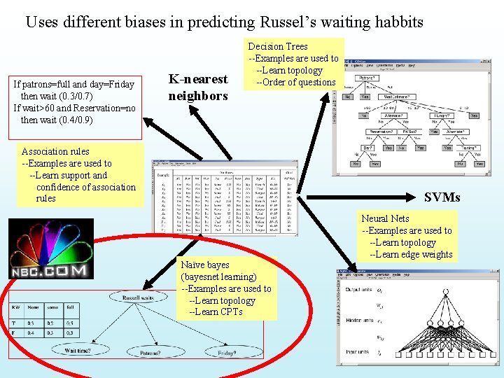
A classification learning example Predicting when Rusell will wait for a table --similar to book preferences, predicting credit card fraud, predicting when people are likely to respond to junk mail

Uses different biases in predicting Russel’s waiting habbits If patrons=full and day=Friday then wait (0. 3/0. 7) If wait>60 and Reservation=no then wait (0. 4/0. 9) K-nearest neighbors Decision Trees --Examples are used to --Learn topology --Order of questions Association rules --Examples are used to --Learn support and confidence of association rules SVMs Neural Nets --Examples are used to --Learn topology --Learn edge weights Naïve bayes (bayesnet learning) --Examples are used to --Learn topology --Learn CPTs

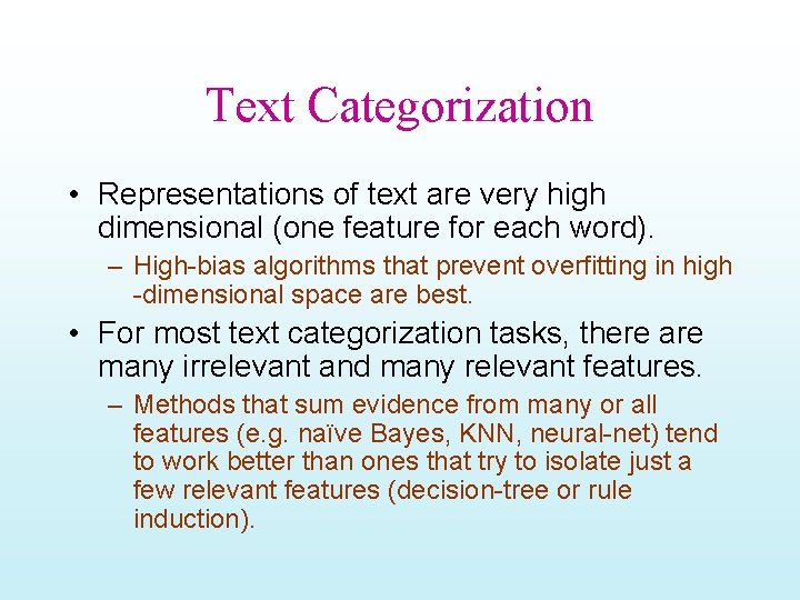
Text Categorization • Representations of text are very high dimensional (one feature for each word). – High-bias algorithms that prevent overfitting in high -dimensional space are best. • For most text categorization tasks, there are many irrelevant and many relevant features. – Methods that sum evidence from many or all features (e. g. naïve Bayes, KNN, neural-net) tend to work better than ones that try to isolate just a few relevant features (decision-tree or rule induction).

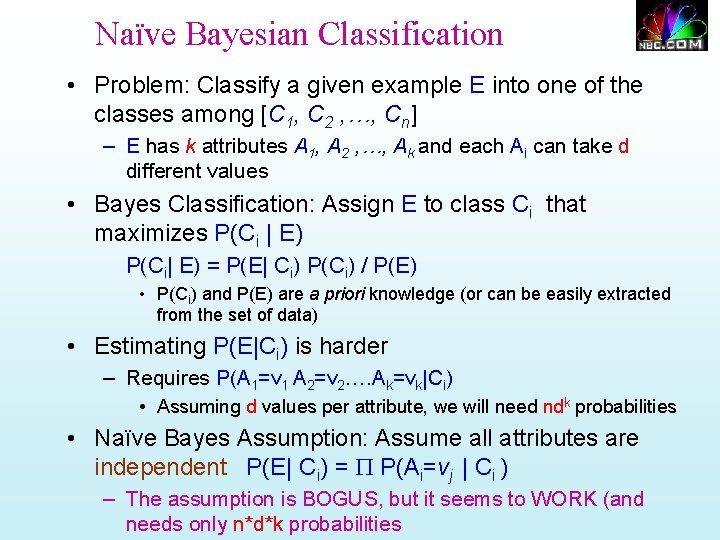
Naïve Bayesian Classification • Problem: Classify a given example E into one of the classes among [C 1, C 2 , …, Cn] – E has k attributes A 1, A 2 , …, Ak and each Ai can take d different values • Bayes Classification: Assign E to class Ci that maximizes P(Ci | E) P(Ci| E) = P(E| Ci) P(Ci) / P(E) • P(Ci) and P(E) are a priori knowledge (or can be easily extracted from the set of data) • Estimating P(E|Ci) is harder – Requires P(A 1=v 1 A 2=v 2…. Ak=vk|Ci) • Assuming d values per attribute, we will need ndk probabilities • Naïve Bayes Assumption: Assume all attributes are independent P(E| Ci) = P P(Ai=vj | Ci ) – The assumption is BOGUS, but it seems to WORK (and needs only n*d*k probabilities

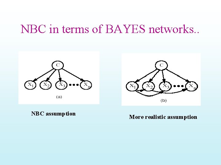
NBC in terms of BAYES networks. . NBC assumption More realistic assumption

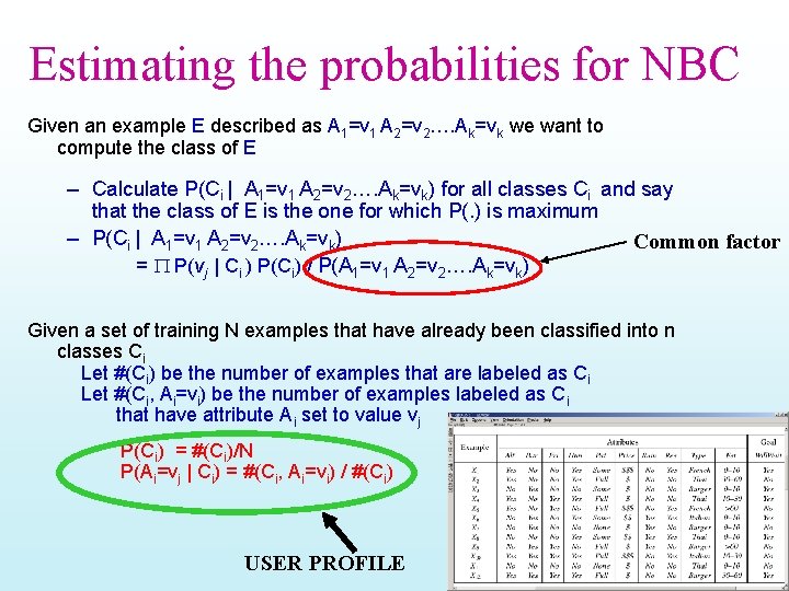
Estimating the probabilities for NBC Given an example E described as A 1=v 1 A 2=v 2…. Ak=vk we want to compute the class of E – Calculate P(Ci | A 1=v 1 A 2=v 2…. Ak=vk) for all classes Ci and say that the class of E is the one for which P(. ) is maximum – P(Ci | A 1=v 1 A 2=v 2…. Ak=vk) Common factor = P P(vj | Ci ) P(Ci) / P(A 1=v 1 A 2=v 2…. Ak=vk) Given a set of training N examples that have already been classified into n classes Ci Let #(Ci) be the number of examples that are labeled as Ci Let #(Ci, Ai=vi) be the number of examples labeled as Ci that have attribute Ai set to value vj P(Ci) = #(Ci)/N P(Ai=vj | Ci) = #(Ci, Ai=vi) / #(Ci) USER PROFILE

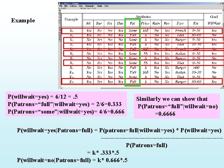
Example P(willwait=yes) = 6/12 =. 5 P(Patrons=“full”|willwait=yes) = 2/6=0. 333 P(Patrons=“some”|willwait=yes)= 4/6=0. 666 Similarly we can show that P(Patrons=“full”|willwait=no) =0. 6666 P(willwait=yes|Patrons=full) = P(patrons=full|willwait=yes) * P(willwait=yes) -----------------------------P(Patrons=full) = k*. 333*. 5 P(willwait=no|Patrons=full) = k* 0. 666*. 5

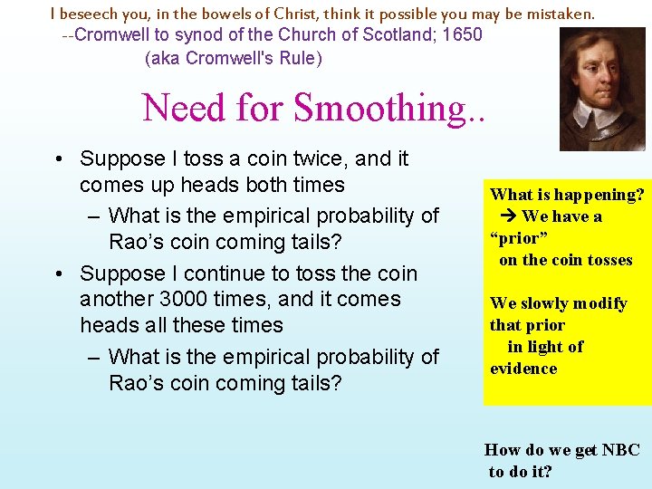
I beseech you, in the bowels of Christ, think it possible you may be mistaken. --Cromwell to synod of the Church of Scotland; 1650 (aka Cromwell's Rule) Need for Smoothing. . • Suppose I toss a coin twice, and it comes up heads both times – What is the empirical probability of Rao’s coin coming tails? • Suppose I continue to toss the coin another 3000 times, and it comes heads all these times – What is the empirical probability of Rao’s coin coming tails? What is happening? We have a “prior” on the coin tosses We slowly modify that prior in light of evidence How do we get NBC to do it?

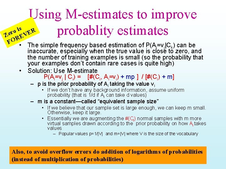
Using M-estimates to improve is R o r probablity estimates Ze REVE FO • The simple frequency based estimation of P(A =v |C ) can be i j k inaccurate, especially when the true value is close to zero, and the number of training examples is small (so the probability that your examples don’t contain rare cases is quite high) • Solution: Use M-estimate P(Ai=vj | Ci) = [#(Ci, Ai=vi) + mp ] / [#(Ci) + m] – p is the prior probability of Ai taking the value vi • If we don’t have any background information, assume uniform probability (that is 1/d if Ai can take d values) – m is a constant—called “equivalent sample size” • If we believe that our sample set is large enough, we can keep m small. Otherwise, keep it large. • Essentially we are augmenting the #(Ci) normal samples with m more virtual samples drawn according to the prior probability on how Ai takes values – Popular values p=1/|V| and m=|V| where V is the size of the vocabulary Also, to avoid overflow errors do addition of logarithms of probabilities (instead of multiplication of probabilities)

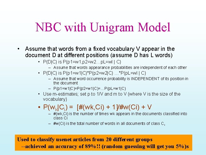
NBC with Unigram Model • Assume that words from a fixed vocabulary V appear in the document D at different positions (assume D has L words) • P(D|C) is P(p 1=w 1, p 2=w 2…p. L=wl | C) – Assume that words appearance probabilities are independent of each other • P(D|C) is P(p 1=w 1|C)*P(p 2=w 2|C) …*P(p. L=wl | C) – Assume that word occurrence probability is INDEPENDENT of its position in the document – P(p 1=w 1|C)=P(p 2=w 1|C)=…P(p. L=w 1|C) • Use m-estimates; set p to 1/V and m to V (where V is the size of the vocabulary) • P(wk|Ci) = [#(wk, Ci) + 1]/#w(Ci) + V – #(wk, Ci) is the number of times wk appears in the documents classified into class Ci – #w(Ci) is the total number of words in all documents of class Ci Used to classify usenet articles from 20 different groups --achieved an accuracy of 89%!! (random guessing will get you 5%)s

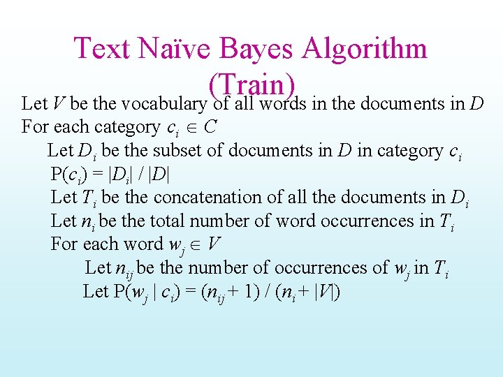
Text Naïve Bayes Algorithm (Train) Let V be the vocabulary of all words in the documents in D For each category ci C Let Di be the subset of documents in D in category ci P(ci) = |Di| / |D| Let Ti be the concatenation of all the documents in Di Let ni be the total number of word occurrences in Ti For each word wj V Let nij be the number of occurrences of wj in Ti Let P(wj | ci) = (nij + 1) / (ni + |V|)

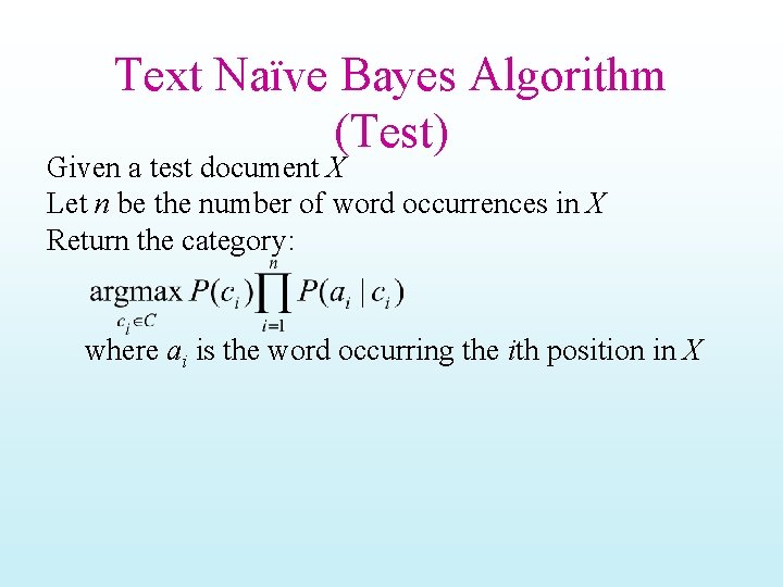
Text Naïve Bayes Algorithm (Test) Given a test document X Let n be the number of word occurrences in X Return the category: where ai is the word occurring the ith position in X

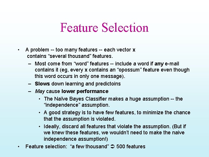
Feature Selection • • A problem -- too many features -- each vector x contains “several thousand” features. – Most come from “word” features -- include a word if any e-mail contains it (eg, every x contains an “opossum” feature even though this word occurs in only one message). – Slows down learning and predictoins – May cause lower performance • The Naïve Bayes Classifier makes a huge assumption -- the “independence” assumption. • A good strategy is to have few features, to minimize the chance that the assumption is violated. • Ideally, discard all features that violate the assumption. (But if we knew these features, we wouldn’t need to make the naive independence assumption!) Feature selection: “a few thousand” 500 features

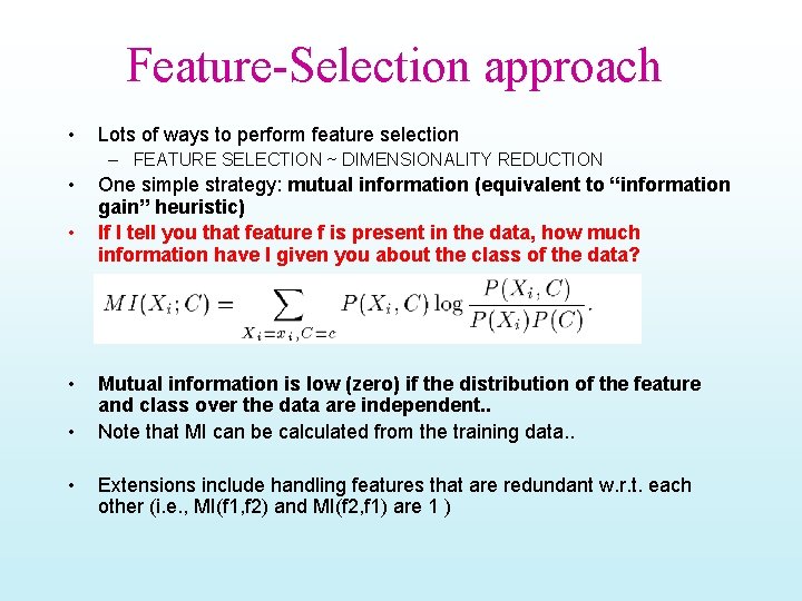
Feature-Selection approach • Lots of ways to perform feature selection – FEATURE SELECTION ~ DIMENSIONALITY REDUCTION • • • One simple strategy: mutual information (equivalent to “information gain” heuristic) If I tell you that feature f is present in the data, how much information have I given you about the class of the data? Mutual information is low (zero) if the distribution of the feature and class over the data are independent. . Note that MI can be calculated from the training data. . Extensions include handling features that are redundant w. r. t. each other (i. e. , MI(f 1, f 2) and MI(f 2, f 1) are 1 )

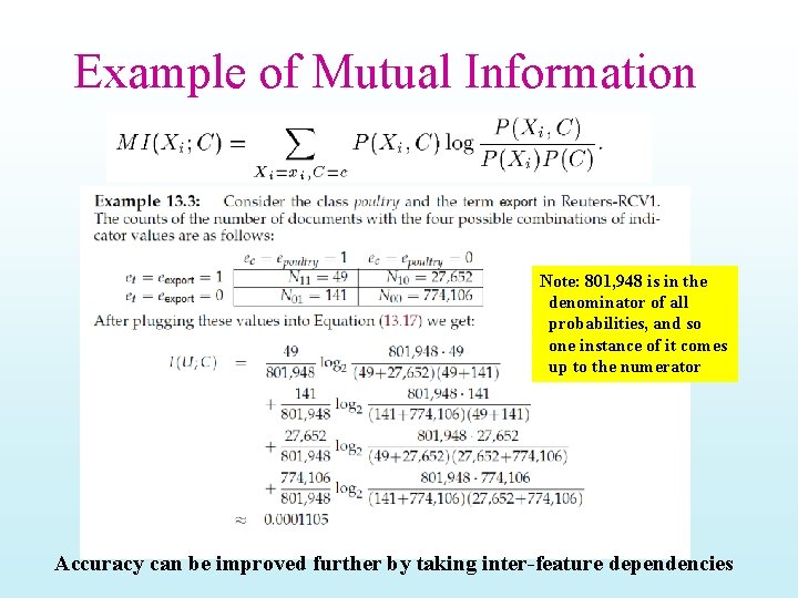
Example of Mutual Information Note: 801, 948 is in the denominator of all probabilities, and so one instance of it comes up to the numerator Accuracy can be improved further by taking inter-feature dependencies

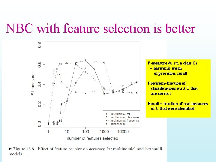
NBC with feature selection is better F-measure (w. r. t. a class C) = harmonic mean of precision, recall Precision=fraction of classifications w. r. t C that are correct Recall = fraction of real instances of C that were identified

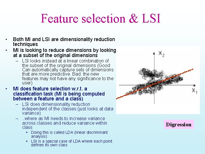
Feature selection & LSI • • Both MI and LSI are dimensionality reduction techniques MI is looking to reduce dimensions by looking at a subset of the original dimensions – LSI looks instead at a linear combination of the subset of the original dimensions (Good: Can automatically capture sets of dimensions that are more predictive. Bad: the new features may not have any significance to the user) • MI does feature selection w. r. t. a classification task (MI is being computed between a feature and a class) – LSI does dimensionality reduction independent of the classes (just looks at data variance) –. . where as MI needs to increase variance across classes and reduce variance within class • Doing this is called LDA (linear discriminant analysis) • LSI is a special case of LDA where each point defines its own class Digression

Experiments • 1789 hand-tagged e-mail messages – 1578 junk – 211 legit • Split into… – 1528 training messages (86%) – 251 testing messages (14%) – Similar to experiment described in Ad. Eater lecture, except messages are not randomly split. This is unfortunate -maybe performance is just a fluke. • Training phase: Compute Pr[X=x|C=junk], Pr[X=x], and P[C=junk] from training messages • Testing phase: Compute Pr[C=junk|X=x] for each training message x. Predict “junk” if Pr[C=junk|X=x]>0. 999. Record mistake/correct answer in confusion matrix.

How Well (and WHY) DOES NBC WORK? • Naïve bayes classifier is darned easy to implement • Good learning speed, classification speed • Modest space storage • Supports incrementality – Recommendations re-done as more attribute values of the new item become known. • It seems to work very well in many scenarios – Peter Norvig, the director of Machine Learning at GOOGLE said, when asked about what sort of technology they use “Naïve bayes” • But WHY? – [Domingos/Pazzani; 1996] showed that NBC has much wider ranges of applicability than previously thought (despite using the independence assumption) – classification accuracy is different from probability estimate accuracy • Notice that normal classification application don’t quite care about the actual probability; only which probability is the highest – Exception is Cost-based learning—suppose false positives and false negatives have different costs… » E. g. Sahami et al consider a message to be spam only if Spam class probability is >. 9 (so they are using incorrect NBC estimates here)