TALYS a tool to go from theoretical modeling

TALYS: a tool to go from theoretical modeling of nuclear reactions to evaluations Part I EJC 2014 – S. Hilaire & The TALYS Team – 30/09/2014

Content - Introduction TODAY - General features about nuclear reactions • Time scales and associated models • Types of data needed • Data format = f (users) - Nuclear Models • • • Basic structure properties Optical model Pre-equilibrium model Compound Nucleus model Miscellaneous : level densities, fission, capture - From in depth analysis to large scale production with TALYS • General features about TALYS • Fine tuning and accuracy • Global systematic approaches - What remains to be done ? TOMORROW

INTRODUCTION CEA | 10 AVRIL 2012

Why do we need nuclear data and how much accurate ? Nuclear data needed for Understanding basic reaction mechanism between particles and nuclei Astrophysical applications (Age of the Galaxy, element abundances …) Good accuracy if possible good understanding or room for improvements Existing or future nuclear reactor simulations Medical applications, oil well logging, waste transmutation, fusion, … Finite number of experimental data (price, safety or counting rates) Complete measurements restricted to low energies ( < 1 Me. V) to scarce nuclei Predictive & Robust Nuclear models (codes) are essential

Why do we need nuclear data and how much accurate ? Nuclear data needed for Understanding basic reaction mechanism between particles and nuclei Astrophysical applications (Age of the Galaxy, element abundances …) Existing or accuracy future nuclear reactor Good if possible goodsimulations understanding or room for improvements Medical applications, oil well logging, waste transmutation, Predictive power important sound physics (first principles) fusion, … Finite number of experimental data (price, safety or counting rates) Complete measurements restricted to low energies ( < 1 Me. V) to scarce nuclei Predictive & Robust Nuclear models (codes) are essential

Why do we need nuclear data and how much accurate ? Nuclear data needed for Understanding basic reaction mechanism between particles and nuclei Astrophysical applications (Age of the Galaxy, element abundances …) Existing or future nuclear reactor simulations Medical applications, oil well required logging, waste transmutation, fusion, … Good (Excellent) accuracy reproduction of data, safety power less important Reproductive Finite Predictive number of experimental data (price, safetypower or counting rates) Complete measurements restricted to low energies ( < 1 Me. V) to scarce nuclei Predictive & Robust Nuclear models (codes) are essential

Why do we need nuclear data and how much accurate ? Nuclear data needed for Understanding basic reaction mechanism between particles and nuclei Astrophysical applications (Age of the Galaxy, element abundances …) Existing or future nuclear reactor simulations Medical applications, oil well logging, waste transmutation, fusion, … Finite Good number of experimental data (price, safety or counting rates) accuracy required reproduction of data Predictive power less important Reproductive power Complete measurements restricted to low energies ( < 1 Me. V) to scarce nuclei Predictive & Robust Nuclear models (codes) are essential

Why do we need nuclear data and how much accurate ? Nuclear data needed for Understanding basic reaction mechanism between particles and nuclei Astrophysical applications (Age of the Galaxy, element abundances …) Existing or future nuclear reactor simulations Medical applications, oil well logging, waste transmutation, fusion, … But Finite number of experimental data (price, safety or counting rates) Complete measurements restricted to low energies ( < 1 Me. V) to scarce nuclei Predictive & Robust Nuclear models (codes) are essential

GENERAL FEATURES ABOUT NUCLEAR REACTIONS CEA | 10 AVRIL 2012 | PAGE 9 18 SEPTEMBRE 2021

Content - Introduction - General features about nuclear reactions • Time scales and associated models • Types of data needed • Data format = f (users) - Nuclear Models • • • Basic structure properties Optical model Pre-equilibrium model Compound Nucleus model Miscellaneous : level densities, fission, capture - From in depth analysis to large scale production with TALYS • General features about TALYS • Fine tuning and accuracy • Global systematic approaches - What remains to be done ?

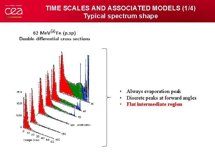
TIME SCALES AND ASSOCIATED MODELS (1/4) Typical spectrum shape • Always evaporation peak • Discrete peaks at forward angles • Flat intermediate region

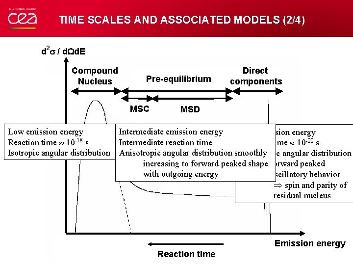
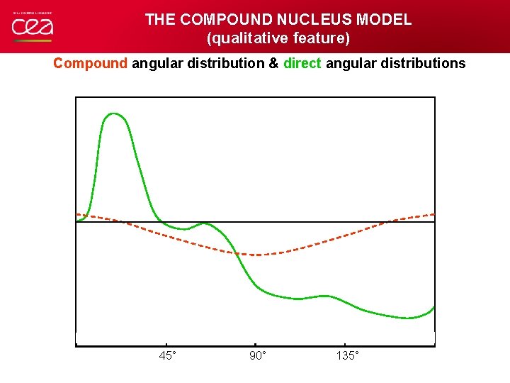
TIME SCALES AND ASSOCIATED MODELS (2/4) d 2 / d. Wd. E Compound Nucleus Pre-equilibrium MSC Direct components MSD Low emission energy Intermediate emission energy High emission energy Reaction time 10 -18 s Intermediate reaction time Reaction time 10 -22 s Isotropic angular distribution Anisotropic angular distribution smoothly Anisotropic angular distribution increasing to forward peaked shape- forward peaked with outgoing energy - oscillatory behavior spin and parity of residual nucleus Emission energy Reaction time

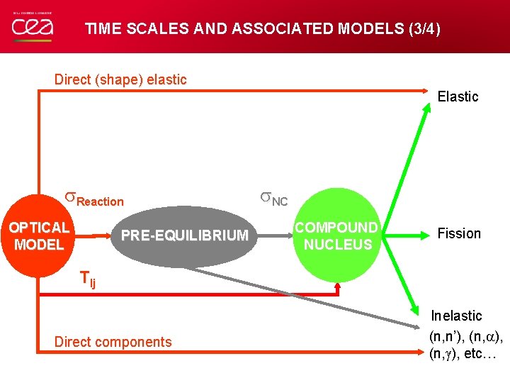
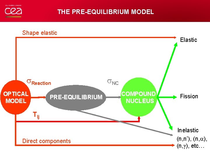
TIME SCALES AND ASSOCIATED MODELS (3/4) Direct (shape) elastic Elastic Reaction OPTICAL MODEL PRE-EQUILIBRIUM NC COMPOUND NUCLEUS Fission Tlj Direct components Inelastic (n, n’), (n, ), etc…

TIME SCALES AND ASSOCIATED MODELS (4/4)

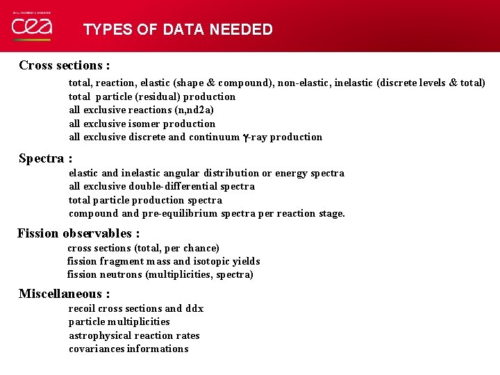
TYPES OF DATA NEEDED Cross sections : total, reaction, elastic (shape & compound), non-elastic, inelastic (discrete levels & total) total particle (residual) production all exclusive reactions (n, nd 2 a) all exclusive isomer production all exclusive discrete and continuum g-ray production Spectra : elastic and inelastic angular distribution or energy spectra all exclusive double-differential spectra total particle production spectra compound and pre-equilibrium spectra per reaction stage. Fission observables : cross sections (total, per chance) fission fragment mass and isotopic yields fission neutrons (multiplicities, spectra) Miscellaneous : recoil cross sections and ddx particle multiplicities astrophysical reaction rates covariances informations

DATA FORMAT • Trivial for basic nuclear science : x, y, (z) file • Complicated (even crazy) for data production issues : ENDF file

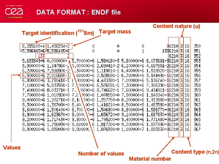
DATA FORMAT : ENDF file • Target Trivialidentification for basic ( mass x, y, (z) file Sm) : Target nuclear 151 science Content nature ( ) • Complicated (even crazy) for data production issues : ENDF file Values Number of values Content type (n, 2 n) Material number

NUCLEAR MODELS CEA | 10 AVRIL 2012 | PAGE 18 18 SEPTEMBRE 2021

Content - Introduction - General features about nuclear reactions • Time scales and associated models • Types of data needed • Data format = f (users) - Nuclear Models • • • Basic structure properties Optical model Pre-equilibrium model Compound Nucleus model Miscellaneous : level densities, fission, capture - From in depth analysis to large scale production with TALYS • General features about TALYS • Fine tuning and accuracy • Global systematic approaches - What remains to be done ?

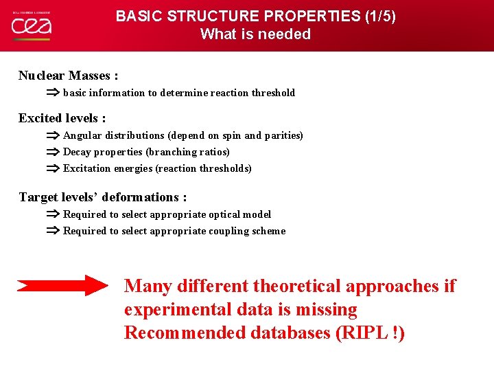
BASIC STRUCTURE PROPERTIES (1/5) What is needed Nuclear Masses : basic information to determine reaction threshold Excited levels : Angular distributions (depend on spin and parities) Decay properties (branching ratios) Excitation energies (reaction thresholds) Target levels’ deformations : Required to select appropriate optical model Required to select appropriate coupling scheme Many different theoretical approaches if experimental data is missing Recommended databases (RIPL !)

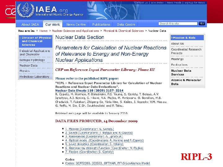
RIPL-3

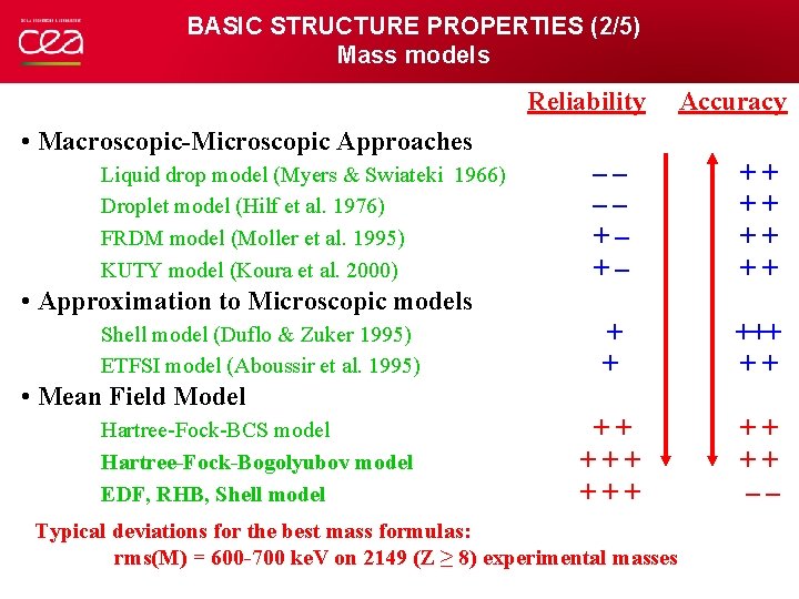
BASIC STRUCTURE PROPERTIES (2/5) Mass models Reliability Accuracy • Macroscopic-Microscopic Approaches Liquid drop model (Myers & Swiateki 1966) Droplet model (Hilf et al. 1976) FRDM model (Moller et al. 1995) KUTY model (Koura et al. 2000) –– –– +– +– ++ ++ ++ +++ ++ ++ –– • Approximation to Microscopic models Shell model (Duflo & Zuker 1995) ETFSI model (Aboussir et al. 1995) • Mean Field Model Hartree-Fock-BCS model Hartree-Fock-Bogolyubov model EDF, RHB, Shell model Typical deviations for the best mass formulas: rms(M) = 600 -700 ke. V on 2149 (Z ≥ 8) experimental masses

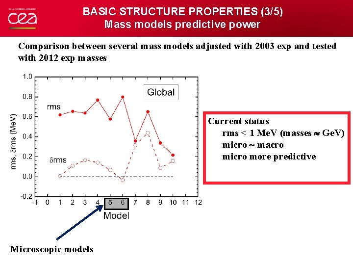
BASIC STRUCTURE PROPERTIES (3/5) Mass models predictive power Comparison between several mass models adjusted with 2003 exp and tested with 2012 exp masses Current status rms < 1 Me. V (masses Ge. V) micro macro micro more predictive Microscopic models

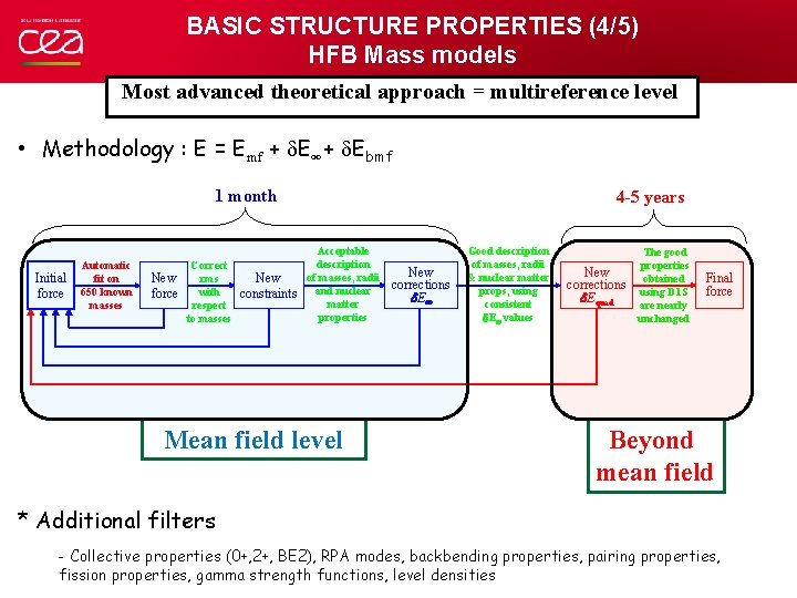
BASIC STRUCTURE PROPERTIES (4/5) HFB Mass models Most advanced theoretical approach = multireference level • Methodology : E = Emf + d. E∞+ d. Ebmf 1 month Initial force Automatic fit on 650 known masses New force Correct rms with respect to masses New constraints 4 -5 years Acceptable description of masses, radii and nuclear matter properties Mean field level New corrections d. E Good description of masses, radii & nuclear matter props, using consistent E values New corrections d. Equad The good properties obtained using D 1 S are nearly unchanged Final force Beyond mean field * Additional filters - Collective properties (0+, 2+, BE 2), RPA modes, backbending properties, pairing properties, fission properties, gamma strength functions, level densities

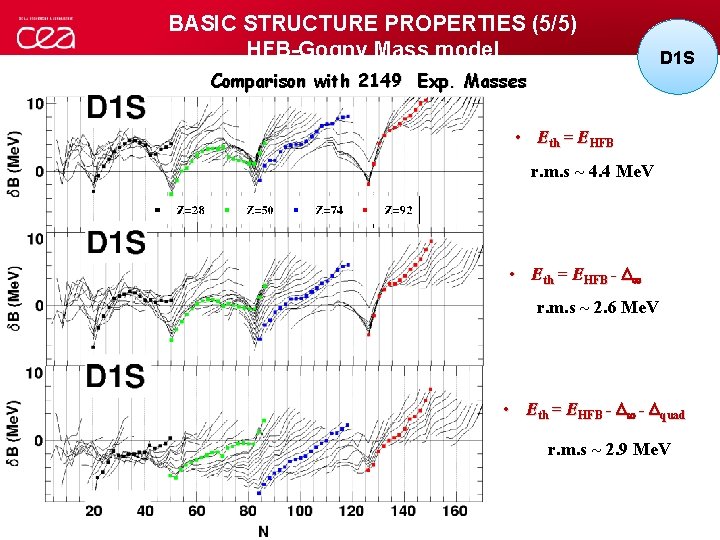
BASIC STRUCTURE PROPERTIES (5/5) HFB-Gogny Mass model Comparison with 2149 Exp. Masses D 1 S • Eth = EHFB r. m. s ~ 4. 4 Me. V • Eth = EHFB - D r. m. s ~ 2. 6 Me. V • Eth = EHFB - Dquad r. m. s ~ 2. 9 Me. V

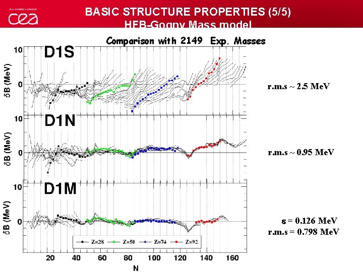
BASIC STRUCTURE PROPERTIES (5/5) HFB-Gogny Mass model Comparison with 2149 Exp. Masses r. m. s ~ 2. 5 Me. V r. m. s ~ 0. 95 Me. V e = 0. 126 Me. V r. m. s = 0. 798 Me. V

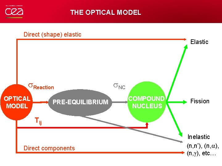
THE OPTICAL MODEL Direct (shape) elastic Elastic Reaction OPTICAL MODEL PRE-EQUILIBRIUM NC COMPOUND NUCLEUS Fission Tlj Direct components Inelastic (n, n’), (n, ), etc…

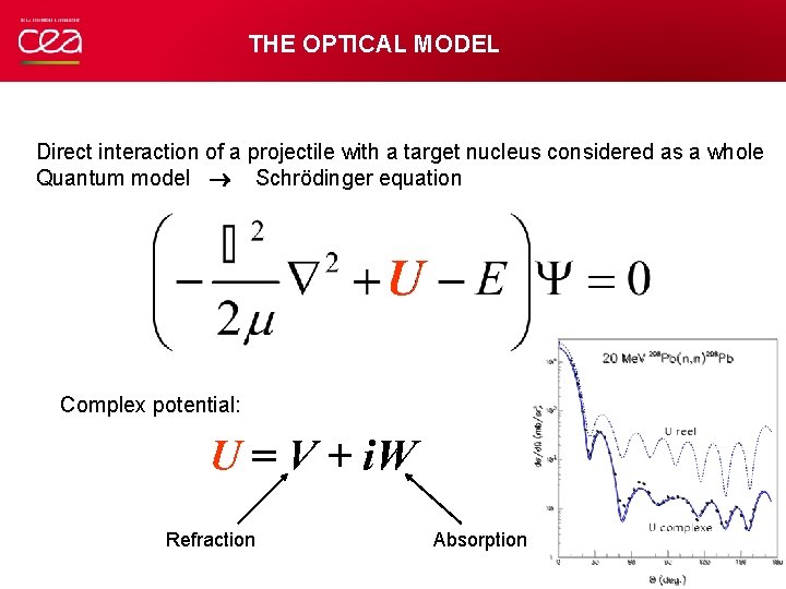
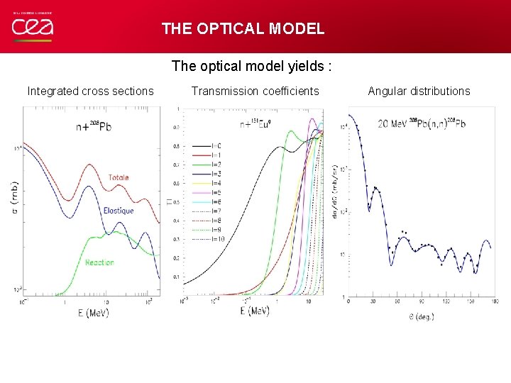
THE OPTICAL MODEL Direct interaction of a projectile with a target nucleus considered as a whole Quantum model Schrödinger equation U Complex potential: U = V + i. W Refraction Absorption

THE OPTICAL MODEL The optical model yields : Integrated cross sections Transmission coefficients Angular distributions

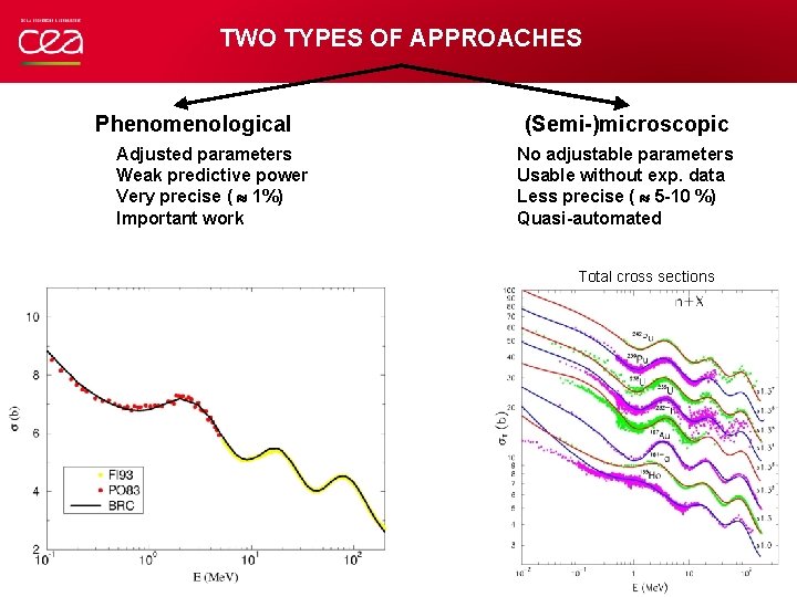
TWO TYPES OF APPROACHES Phenomenological Adjusted parameters Weak predictive power Very precise ( 1%) Important work (Semi-)microscopic No adjustable parameters Usable without exp. data Less precise ( 5 -10 %) Quasi-automated Total cross sections

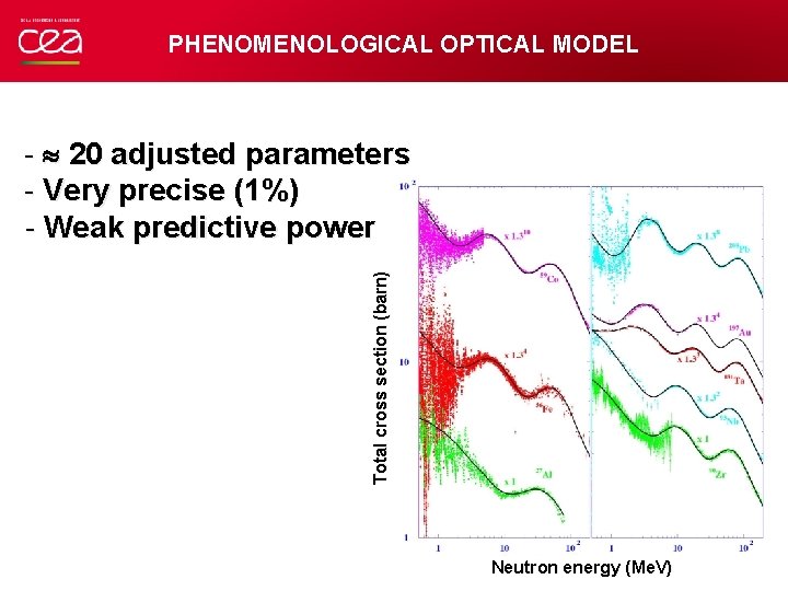
PHENOMENOLOGICAL OPTICAL MODEL Total cross section (barn) - 20 adjusted parameters - Very precise (1%) - Weak predictive power Neutron energy (Me. V)

PHENOMENOLOGICAL OPTICAL MODEL [ ] [ W (E) f(r, R , a ) + W (E) g(r, R , a ) ] U(r, E) = V(E, r)V+ i W(E, r) f(r, RV, a. V) + VS(E) g(r, RS, a. S) V(E) V V V S S Well depths (Me. V) +i f(r, R, a)= -1 1+exp((r-R)/a) Incident energy (Me. V) g(r, R, a) = - df/dr S

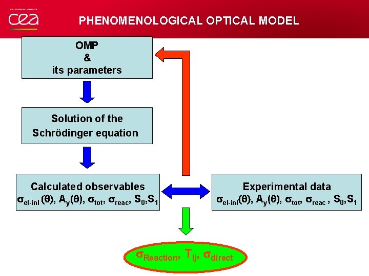
PHENOMENOLOGICAL OPTICAL MODEL OMP & its parameters Solution of the Schrödinger equation Calculated observables el-inl q , Ay(q), tot, reac, S 0, S 1 Experimental data el-inl q , Ay(q), tot, reac , S 0, S 1 Reaction, Tlj, direct

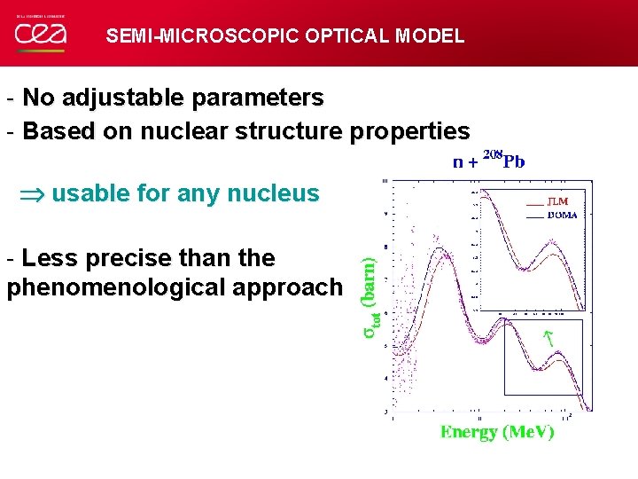
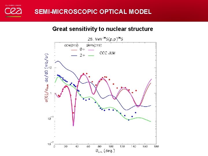
SEMI-MICROSCOPIC OPTICAL MODEL - No adjustable parameters - Based on nuclear structure properties usable for any nucleus - Less precise than the phenomenological approach

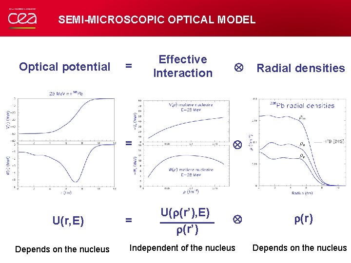
SEMI-MICROSCOPIC OPTICAL MODEL Optical potential = Effective Interaction = U(r, E) Depends on the nucleus = Radial densities U(r(r’), E) r(r’) Independent of the nucleus r(r) Depends on the nucleus

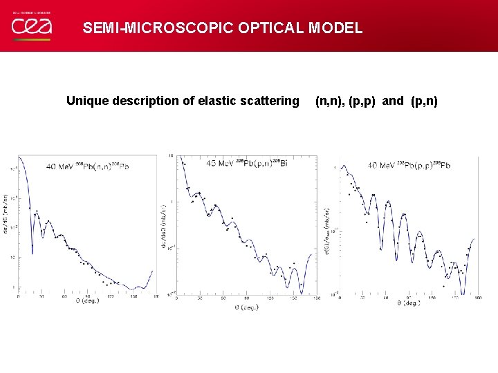
SEMI-MICROSCOPIC OPTICAL MODEL Unique description of elastic scattering (n, n), (p, p) and (p, n)

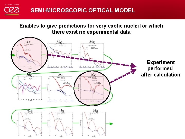
SEMI-MICROSCOPIC OPTICAL MODEL Enables to give predictions for very exotic nuclei for which there exist no experimental data Experiment performed after calculation

SEMI-MICROSCOPIC OPTICAL MODEL Great sensitivity to nuclear structure

THE PRE-EQUILIBRIUM MODEL Shape elastic Elastic Reaction OPTICAL MODEL PRE-EQUILIBRIUM NC COMPOUND NUCLEUS Fission Tlj Direct components Inelastic (n, n’), (n, ), etc…

TIME SCALES AND ASSOCIATED MODELS (1/4) Typical spectrum shape • Always evaporation peak • Discrete peaks at forward angles • Flat intermediate region

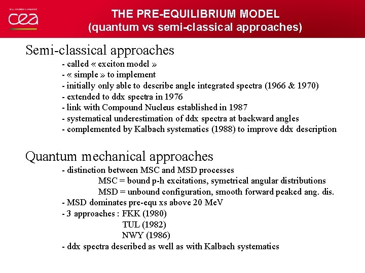
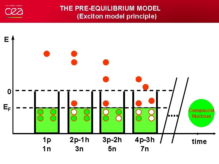
THE PRE-EQUILIBRIUM MODEL (quantum vs semi-classical approaches) Semi-classical approaches - called « exciton model » - « simple » to implement - initially only able to describe angle integrated spectra (1966 & 1970) - extended to ddx spectra in 1976 - link with Compound Nucleus established in 1987 - systematical underestimation of ddx spectra at backward angles - complemented by Kalbach systematics (1988) to improve ddx description Quantum mechanical approaches - distinction between MSC and MSD processes MSC = bound p-h excitations, symetrical angular distributions MSD = unbound configuration, smooth forward peaked ang. dis. - MSD dominates pre-equ xs above 20 Me. V - 3 approaches : FKK (1980) - 3 approaches : TUL (1982) - 3 approaches : NWY (1986) - ddx spectra described as well as with Kalbach systematics

THE PRE-EQUILIBRIUM MODEL (Exciton model principle) E 0 EF Compound Nucleus 1 p 1 n 2 p-1 h 3 n 3 p-2 h 5 n 4 p-3 h 7 n time

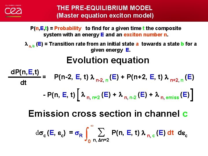
THE PRE-EQUILIBRIUM MODEL (Master equation exciton model) P(n, E, t) = Probability Probabilité to find for a given time t the composite system with an energy E and an exciton number n. l a, b (E) = Transition rate from an initial state a towards a state b for a given energy E. Evolution equation d. P(n, E, t) dt = P(n-2, E, t) l n-2, n (E) + P(n+2, E, t) l n+2, n (E) Apparition [ - P(n, Disparition E, t) l n, n+2 (E) + l n, n-2 (E) + l n, emiss (E) Emission cross section in channel c d c (E, ec) = R ∞ S 0 n, Dn=2 P(n, E, t) l n, c (E) dt dec ]

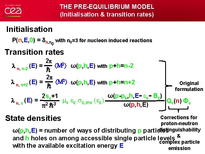
THE PRE-EQUILIBRIUM MODEL (Initialisation & transition rates) Initialisation P(n, E, 0) = n, n 0 with n 0=3 for nucleon induced reactions Transition rates 2 M 2 ω(p, h, E) with p+h=n-2 l n, n-2 (E) = ℏ 2 M 2 ω(p, h, E) with p+h=n+2 l n, n+2 (E) = ℏ l n, c (E) = 2 sc+1 2 ℏ 3 State densities Original formulation ω(p-pb, h, E- ec- Bc) µc ec c, inv (ec) Qc(n) Fc ω(p, h, E) Corrections for proton-neutron distinguishability ω(p, h, E) = number of ways of distributing p particles and h holes on among accessible single particle levels & complex particle with the available excitation energy E emission

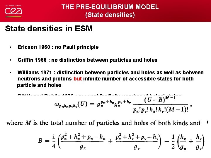
THE PRE-EQUILIBRIUM MODEL (State densities) State densities in ESM • Ericson 1960 : no Pauli principle • Griffin 1966 : no distinction between particles and holes • Williams 1971 : distinction between particles and holes as well as between neutrons and protons but infinite number of accessible states for both particle and holes • Běták and Doběs 1976 : account for finite number of holes’ states • Obložinský 1986 : account for finite number of particles’ states (MSC) • Anzaldo-Meneses 1995 : first order corrections for increasing number of p-h • Hilaire and Koning 1998 : generalized expression in ESM

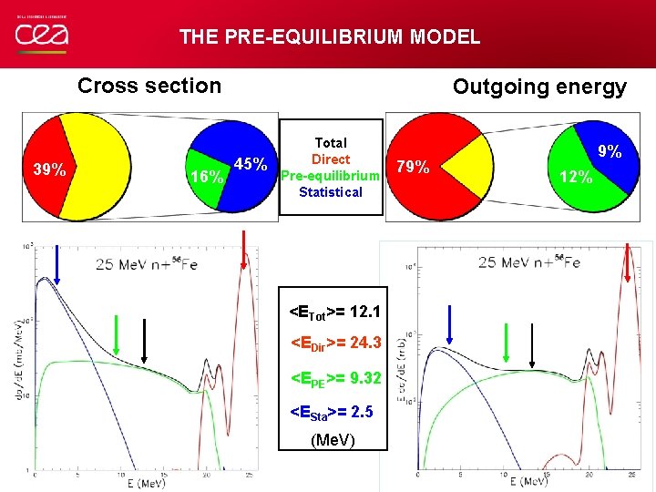
THE PRE-EQUILIBRIUM MODEL Cross section 39% 16% Outgoing energy 45% Total Direct Pre-equilibrium Statistical <ETot>= 12. 1 <EDir>= 24. 3 <EPE>= 9. 32 <ESta>= 2. 5 (Me. V) 79% 9% 12%

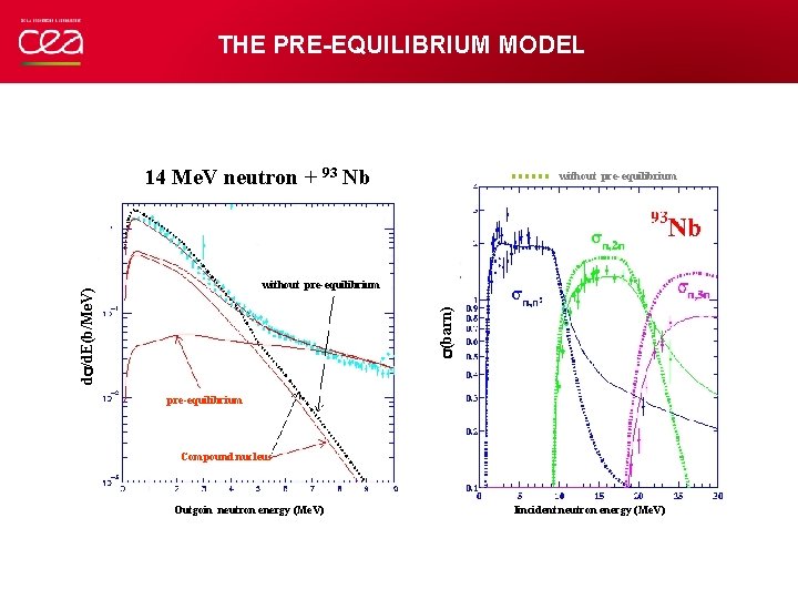
THE PRE-EQUILIBRIUM MODEL 14 Me. V neutron + 93 Nb without pre-equilibrium (barn) d /d. E(b/Me. V) without pre-equilibrium Compound nucleus Outgoin neutron energy (Me. V) Iincident neutron energy (Me. V)

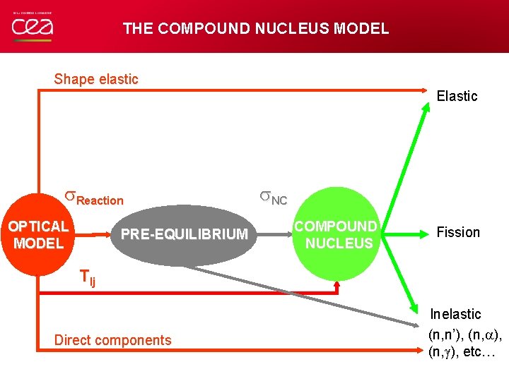
THE COMPOUND NUCLEUS MODEL Shape elastic Elastic Reaction OPTICAL MODEL PRE-EQUILIBRIUM NC COMPOUND NUCLEUS Fission Tlj Direct components Inelastic (n, n’), (n, ), etc…

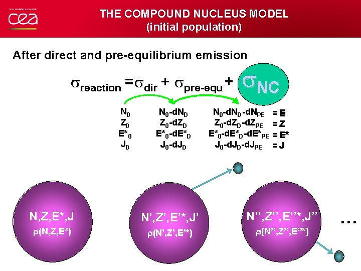
THE COMPOUND NUCLEUS MODEL (initial population) After direct and pre-equilibrium emission reaction = dir + pre-equ + N 0 Z 0 E*0 J 0 N 0 -d. ND Z 0 -d. ZD E*0 -d. E*D J 0 -d. JD NC N 0 -d. ND-d. NPE = E Z 0 -d. ZD-d. ZPE = Z E*0 -d. E*D-d. E*PE = E* J 0 -d. JD-d. JPE = J N, Z, E*, J N’, Z’, E’*, J’ N’’, Z’’, E’’*, J’’ r(N, Z, E*) r(N’, Z’, E’*) r(N’’, Z’’, E’’*) …

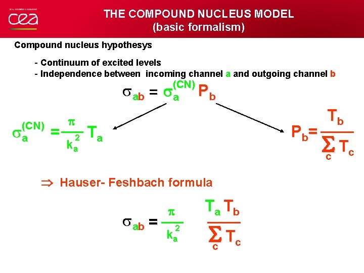
THE COMPOUND NUCLEUS MODEL (basic formalism) Compound nucleus hypothesys - Continuum of excited levels - Independence between incoming channel a and outgoing channel b a b = (CN) a = 2 ka (CN) a Pb P b= Ta Hauser- Feshbach formula a b = Ta Tb 2 ka Sc Tc Tb Sc Tc

THE COMPOUND NUCLEUS MODEL (qualitative feature) Compound angular distribution & direct angular distributions 45° 90° 135°

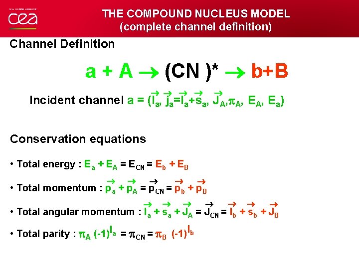
THE COMPOUND NUCLEUS MODEL (complete channel definition) Channel Definition a + A (CN )* b+B Incident channel a = (la, ja=la+sa, JA, A, E A, E a) Conservation equations • Total energy : Ea + EA = ECN = Eb + EB • Total momentum : pa + p. A = p. CN = pb + p. B • Total angular momentum : la + sa + JA = JCN = lb + sb + JB • Total parity : A (-1)la = CN = B (-1) lb

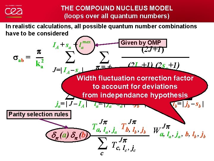
THE COMPOUND NUCLEUS MODEL (loops over all quantum numbers) In realistic calculations, all possible quantum number combinations have to be considered max ab = 2 ka IA + sa + l a S S p S S = Given by OMP (2 J+1) (2 IA+1) (2 sa+1) J=| IA – sa | Width fluctuation correction factor J + IA j a + sa + IB j b + sb to account for Jdeviations from independance hypothesis ja= | J – IA | la= | ja – sa | jb= | J – IB | lb= | jb – sb | Parity selection rules S S T Jp Ta, l , j Tb, l , j W b b a a a, la , ja , b, lb , jb dp (a) dp (b) T Jp Tc, l , j c c c S

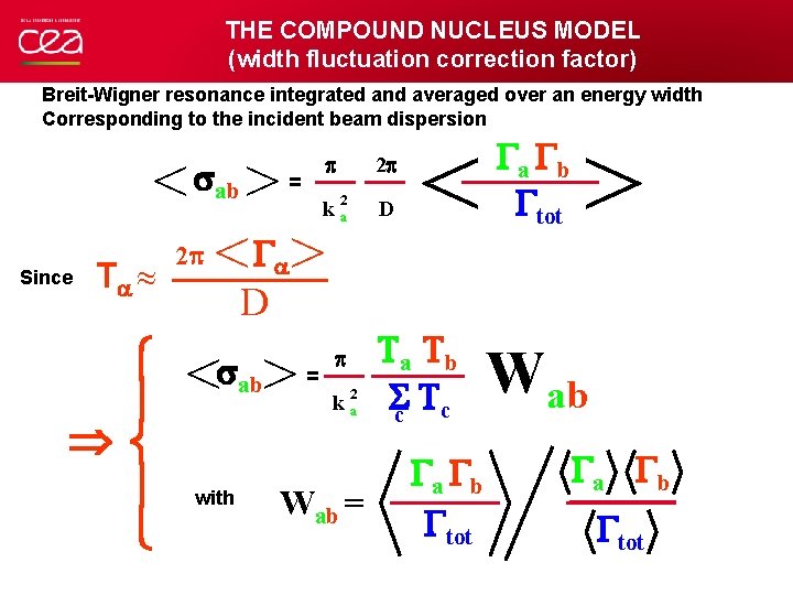
THE COMPOUND NUCLEUS MODEL (width fluctuation correction factor) Breit-Wigner resonance integrated and averaged over an energy width Corresponding to the incident beam dispersion < > 2 < G > = ab Since Ta 2 2 ka D < Ga Gb Gtot > a D < > ab with = k 2 a Wab = Ta Tb Sc Tc Ga Gb Gtot Wab Ga Gb Gtot

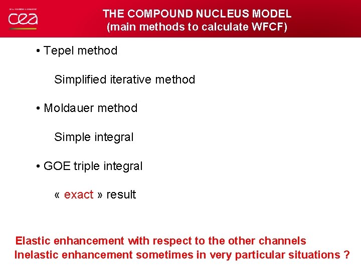
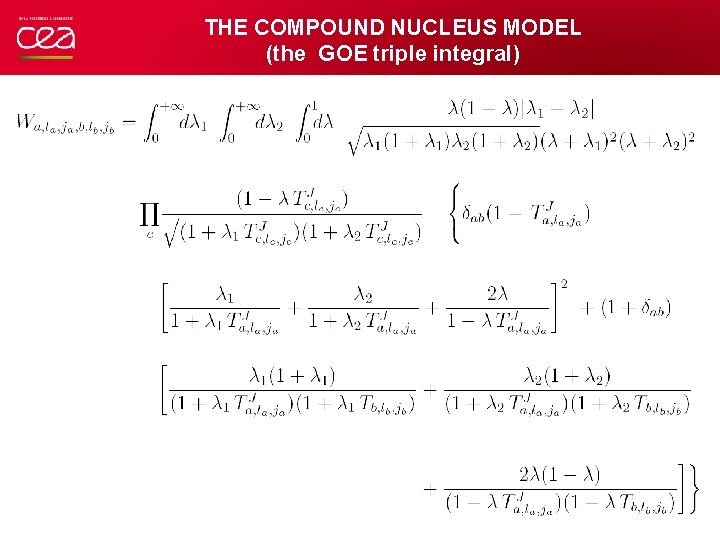
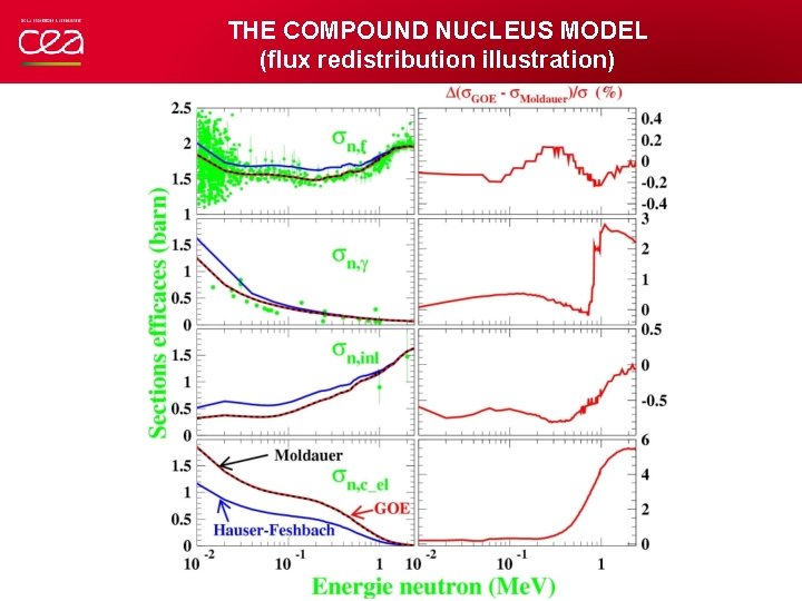
THE COMPOUND NUCLEUS MODEL (main methods to calculate WFCF) • Tepel method Simplified iterative method • Moldauer method Simple integral • GOE triple integral « exact » result Elastic enhancement with respect to the other channels Inelastic enhancement sometimes in very particular situations ?

THE COMPOUND NUCLEUS MODEL (the GOE triple integral)

THE COMPOUND NUCLEUS MODEL (flux redistribution illustration)

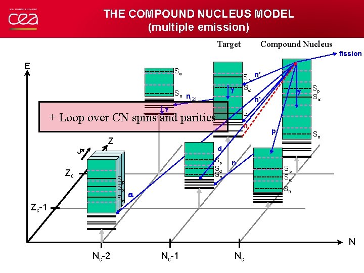
THE COMPOUND NUCLEUS MODEL (multiple emission) Target Compound Nucleus fission E S Sp n’ S g Sn n (2) n’ g n Sp S Sn Sp S n Sn Sp S Sn Sn a Zc-1 p d J Zc Sp S Sn + Loop over CN spins and parities Z g N Nc-2 Nc-1 Nc

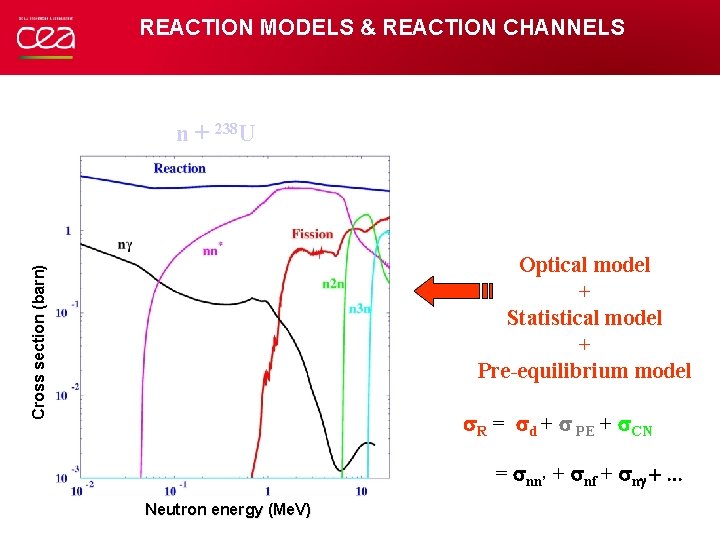
REACTION MODELS & REACTION CHANNELS n + 238 U Cross section (barn) Optical model + Statistical model + Pre-equilibrium model R = d + PE + CN = nn’ + nf + ng +. . . Neutron energy (Me. V)

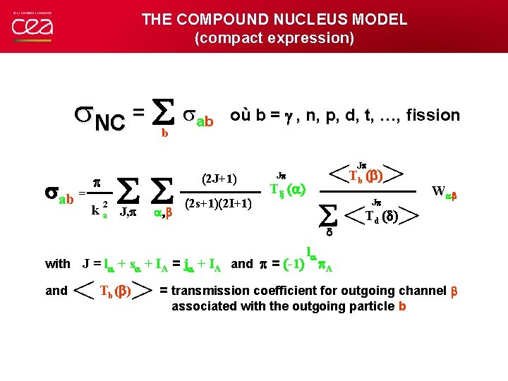
THE COMPOUND NUCLEUS MODEL (compact expression) NC = ab où b = g , n, p, d, t, …, fission b ab = 2 k a J, a, b 2 J+1 2 s+1 2 I+1 < > J Tb b J Tlj a J with J = la + sa + IA = ja + IA and = -1 and < > Tb(b) la Wab Td A = transmission coefficient for outgoing channel b associated with the outgoing particle b

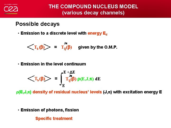
THE COMPOUND NUCLEUS MODEL (various decay channels) Possible decays • Emission to a discrete level with energy Ed < > Tb(b) J = Tlj(b) given by the O. M. P. • Emission in the level continuum < > Tb(b) = E +DE J Tlj(b) r(E, J, ) d. E E r(E, J, ) density of residual nucleus’ levels (J, ) with excitation energy E • Emission of photons, fission Specific treatment