Great Theoretical Ideas In Computer Science Steven Rudich

Great Theoretical Ideas In Computer Science Steven Rudich, Anupam Gupta Lecture 24 CS 15 -251 April 7, 2005 Spring 2005 Carnegie Mellon University Random Walks

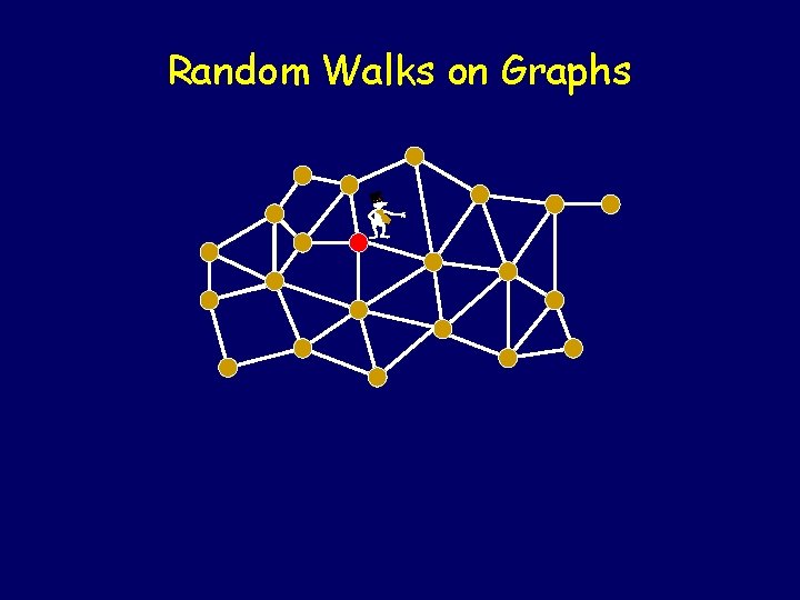
Random Walks on Graphs -

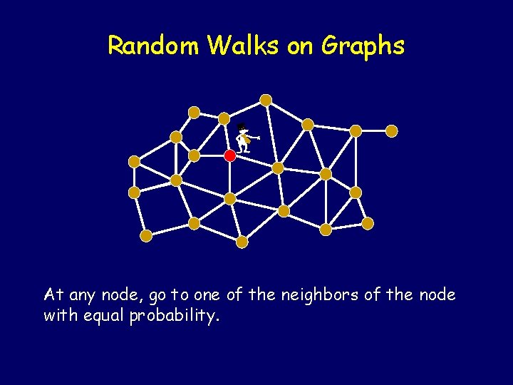
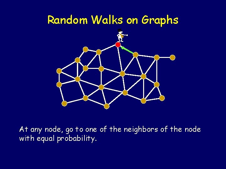
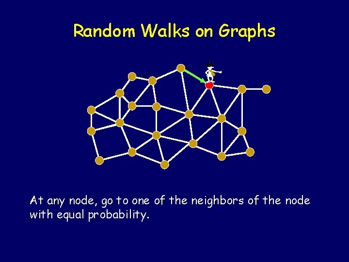
Random Walks on Graphs - At any node, go to one of the neighbors of the node with equal probability.

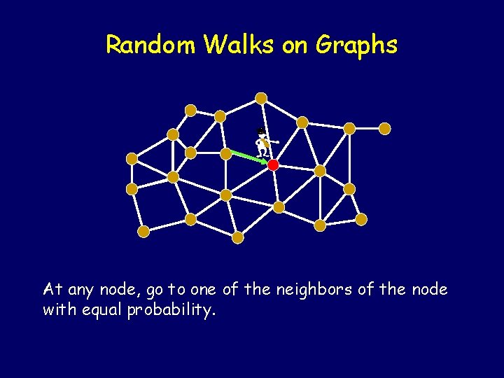
Random Walks on Graphs - At any node, go to one of the neighbors of the node with equal probability.

Random Walks on Graphs - At any node, go to one of the neighbors of the node with equal probability.

Random Walks on Graphs - At any node, go to one of the neighbors of the node with equal probability.

Random Walks on Graphs - At any node, go to one of the neighbors of the node with equal probability.

Let’s start simple… We’ll just walk in a straight line.

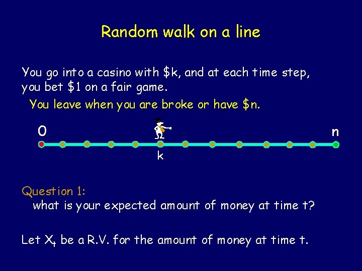
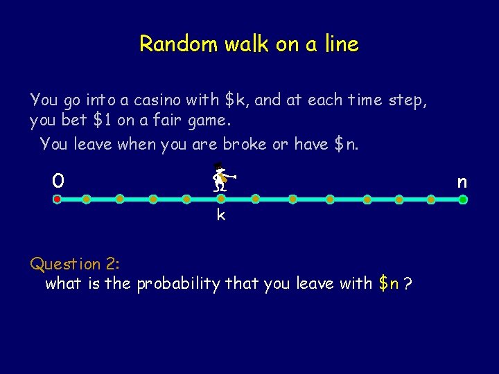
Random walk on a line You go into a casino with $k, and at each time step, you bet $1 on a fair game. You leave when you are broke or have $n. 0 n k Question 1: what is your expected amount of money at time t? Let Xt be a R. V. for the amount of money at time t.

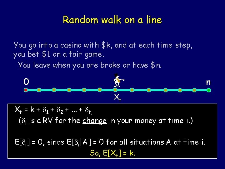
Random walk on a line You go into a casino with $k, and at each time step, you bet $1 on a fair game. You leave when you are broke or have $n. 0 n Xt Xt = k + d 1 + d 2 +. . . + dt, (di is a RV for the change in your money at time i. ) E[di] = 0, since E[di|A] = 0 for all situations A at time i. So, E[Xt] = k.

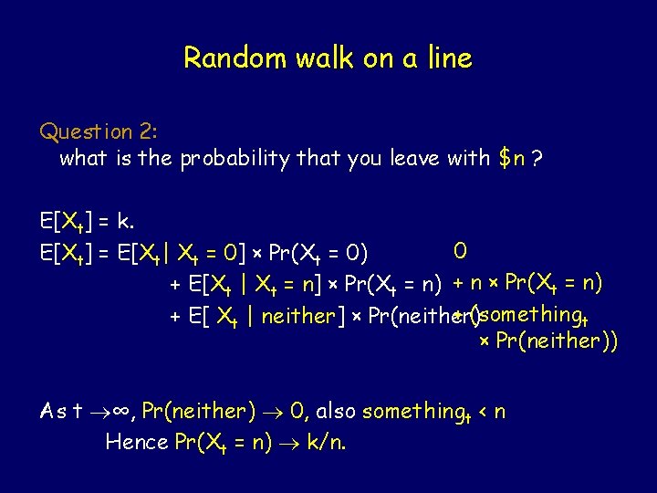
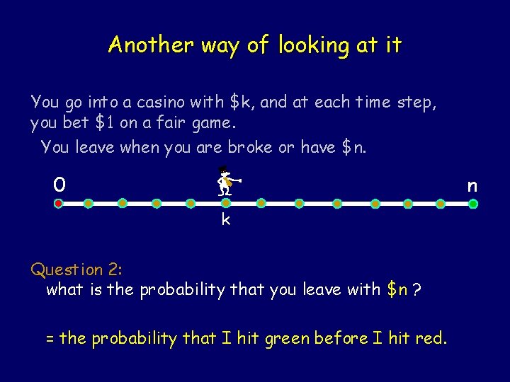
Random walk on a line You go into a casino with $k, and at each time step, you bet $1 on a fair game. You leave when you are broke or have $n. 0 n k Question 2: what is the probability that you leave with $n ?

Random walk on a line Question 2: what is the probability that you leave with $n ? E[Xt] = k. 0 E[Xt] = E[Xt| Xt = 0] × Pr(Xt = 0) + E[Xt | Xt = n] × Pr(Xt = n) + n × Pr(Xt = n) + (somethingt + E[ Xt | neither] × Pr(neither)) As t ∞, Pr(neither) 0, also somethingt < n Hence Pr(Xt = n) k/n.

Another way of looking at it You go into a casino with $k, and at each time step, you bet $1 on a fair game. You leave when you are broke or have $n. 0 n k Question 2: what is the probability that you leave with $n ? = the probability that I hit green before I hit red.

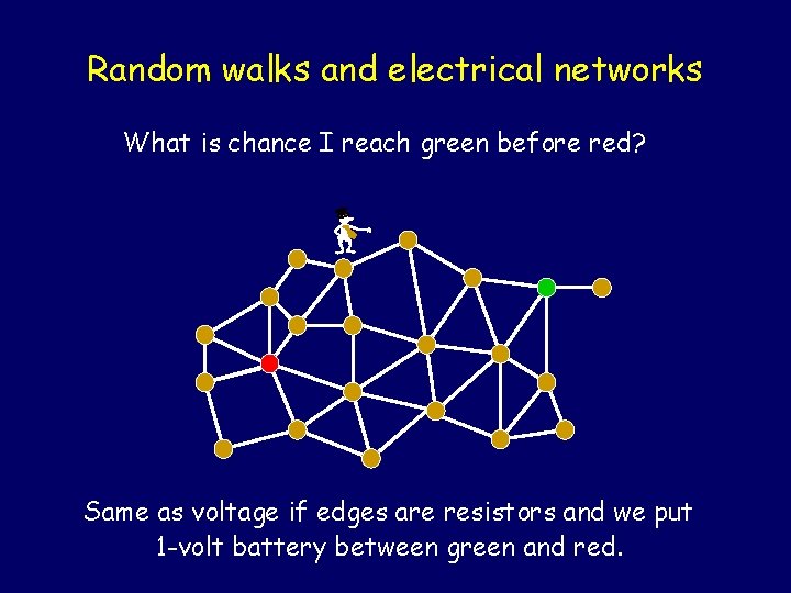
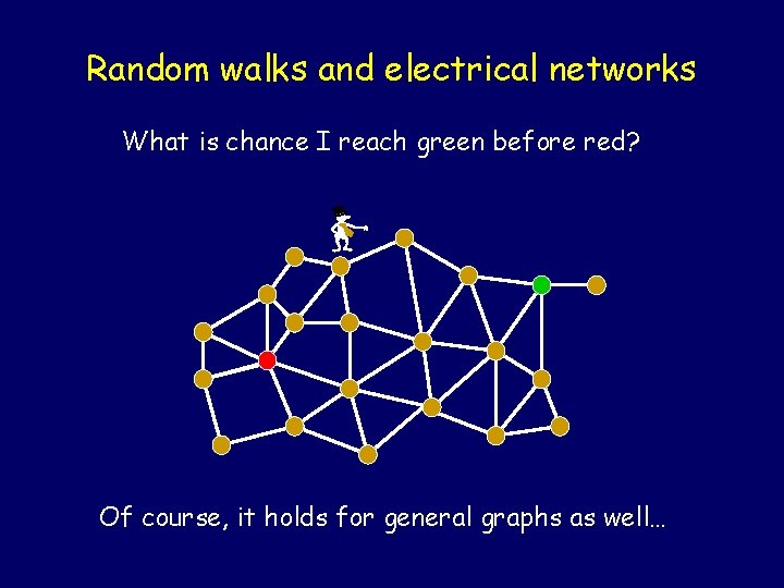
Random walks and electrical networks What is chance I reach green before red? - Same as voltage if edges are resistors and we put 1 -volt battery between green and red.

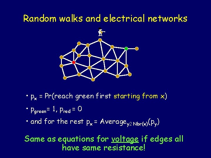
Random walks and electrical networks - • px = Pr(reach green first starting from x) • pgreen= 1, pred = 0 • and for the rest px = Averagey 2 Nbr(x)(py) Same as equations for voltage if edges all have same resistance!

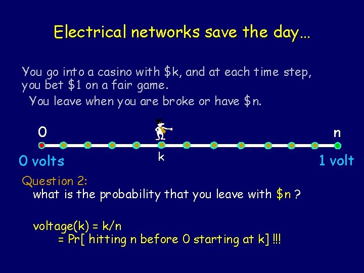
Electrical networks save the day… You go into a casino with $k, and at each time step, you bet $1 on a fair game. You leave when you are broke or have $n. 0 0 volts n k Question 2: what is the probability that you leave with $n ? voltage(k) = k/n = Pr[ hitting n before 0 starting at k] !!! 1 volt

Random walks and electrical networks What is chance I reach green before red? - Of course, it holds for general graphs as well…

Let’s move on to some other questions on general graphs

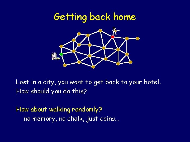
Getting back home - Lost in a city, you want to get back to your hotel. How should you do this? Depth First Search: requires a good memory and a piece of chalk

Getting back home - Lost in a city, you want to get back to your hotel. How should you do this? How about walking randomly? no memory, no chalk, just coins…

Will this work? When will I get home? I have a curfew of 10 PM!

Will this work? Is Pr[ reach home ] = 1? When will I get home? What is E[ time to reach home ]? I have a curfew of 10 PM!

Relax, Bonzo! Yes, Pr[ will reach home ] = 1

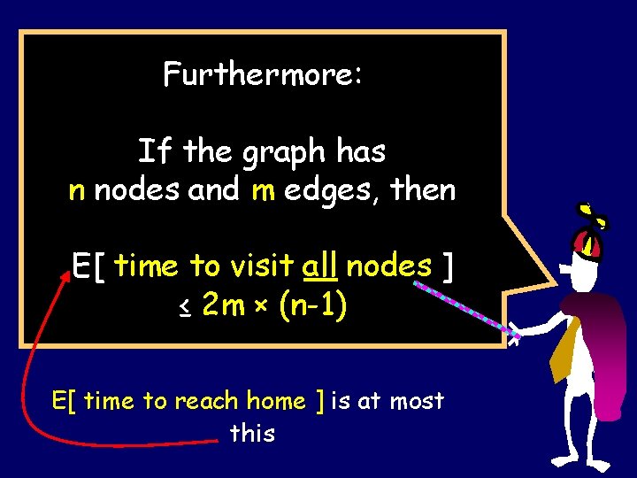
Furthermore: If the graph has n nodes and m edges, then E[ time to visit all nodes ] ≤ 2 m × (n-1) E[ time to reach home ] is at most this

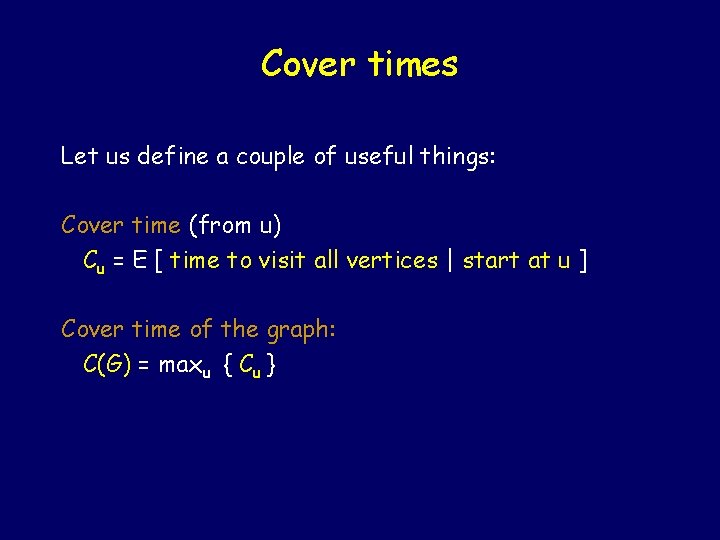
Cover times Let us define a couple of useful things: Cover time (from u) Cu = E [ time to visit all vertices | start at u ] Cover time of the graph: C(G) = maxu { Cu }

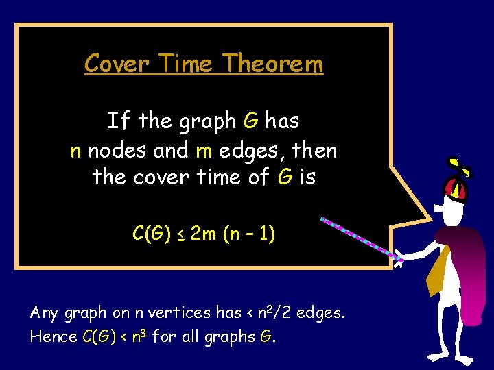
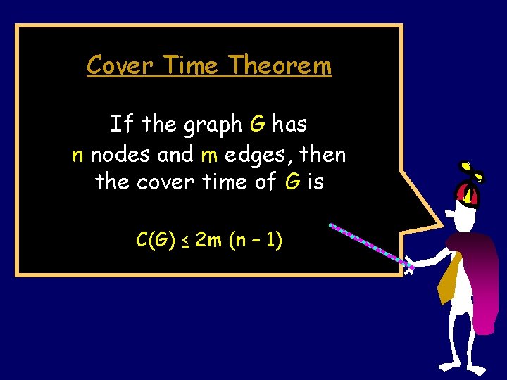
Cover Time Theorem If the graph G has n nodes and m edges, then the cover time of G is C(G) ≤ 2 m (n – 1) Any graph on n vertices has < n 2/2 edges. Hence C(G) < n 3 for all graphs G.

First, let’s prove that Pr[ eventually get home ] = 1

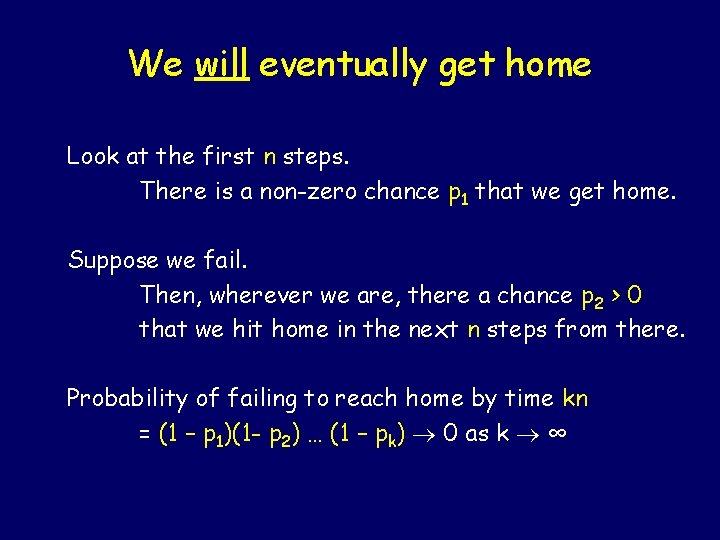
We will eventually get home Look at the first n steps. There is a non-zero chance p 1 that we get home. Suppose we fail. Then, wherever we are, there a chance p 2 > 0 that we hit home in the next n steps from there. Probability of failing to reach home by time kn = (1 – p 1)(1 - p 2) … (1 – pk) 0 as k ∞

In fact Pr[ we don’t get home by 2 k C(G) steps ] ≤ (½)k Recall: C(G) = cover time of G ≤ 2 m(n-1)

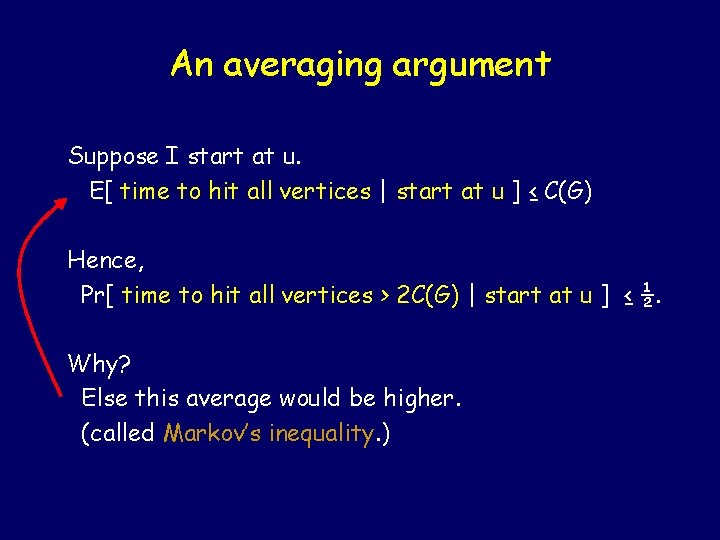
An averaging argument Suppose I start at u. E[ time to hit all vertices | start at u ] ≤ C(G) Hence, Pr[ time to hit all vertices > 2 C(G) | start at u ] ≤ ½. Why? Else this average would be higher. (called Markov’s inequality. )

Markov’s Inequality Random variable X has expectation A = E[X] = E[X | X > 2 A ] Pr[X > 2 A] + E[X | X ≤ 2 A ] Pr[X ≤ 2 A] ≥ E[X | X > 2 A ] Pr[X > 2 A] Also, E[X | X > 2 A] A ≥ 2 A × Pr[X > 2 A] > 2 A ½ ≥ Pr[X > 2 A] Pr[ X exceeds k × expectation ] ≤ 1/k.

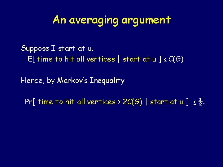
An averaging argument Suppose I start at u. E[ time to hit all vertices | start at u ] ≤ C(G) Hence, by Markov’s Inequality Pr[ time to hit all vertices > 2 C(G) | start at u ] ≤ ½.

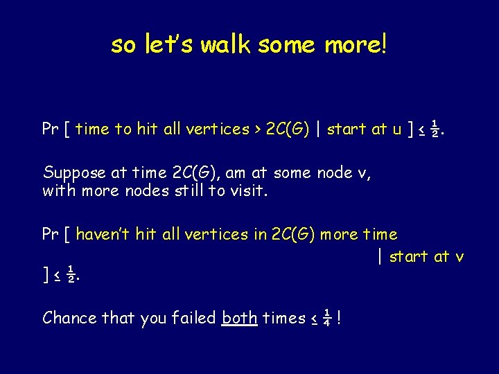
so let’s walk some more! Pr [ time to hit all vertices > 2 C(G) | start at u ] ≤ ½. Suppose at time 2 C(G), am at some node v, with more nodes still to visit. Pr [ haven’t hit all vertices in 2 C(G) more time | start at v ] ≤ ½. Chance that you failed both times ≤ ¼ !

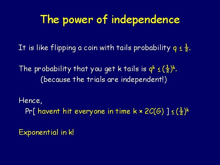
The power of independence It is like flipping a coin with tails probability q ≤ ½. The probability that you get k tails is qk ≤ (½)k. (because the trials are independent!) Hence, Pr[ havent hit everyone in time k × 2 C(G) ] ≤ (½)k Exponential in k!

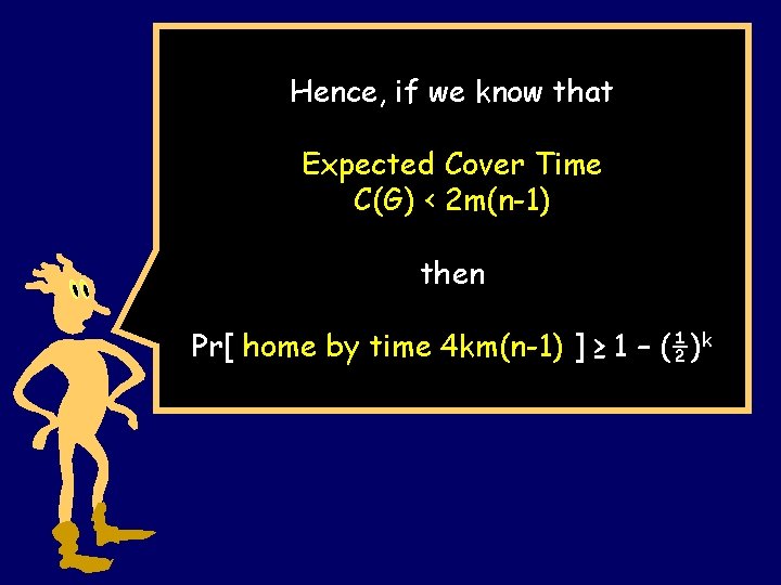
Hence, if we know that Expected Cover Time C(G) < 2 m(n-1) then Pr[ home by time 4 km(n-1) ] ≥ 1 – (½)k

Let us see a cute implication of the fact that we see all the vertices quickly!

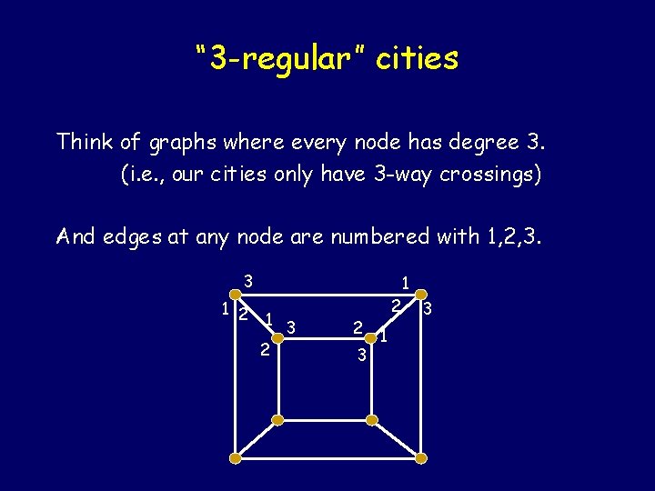
“ 3 -regular” cities Think of graphs where every node has degree 3. (i. e. , our cities only have 3 -way crossings) And edges at any node are numbered with 1, 2, 3. 3 1 2 1 3 2 2 3 2 1 1 3

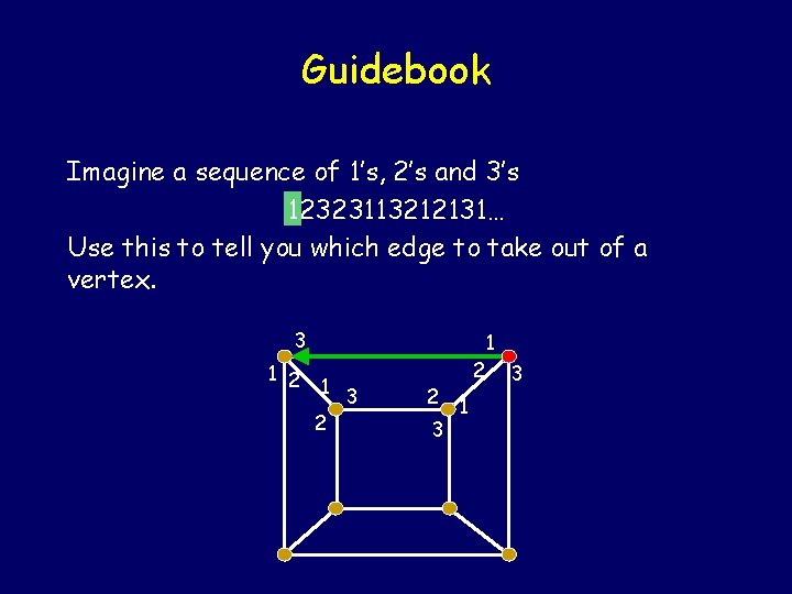
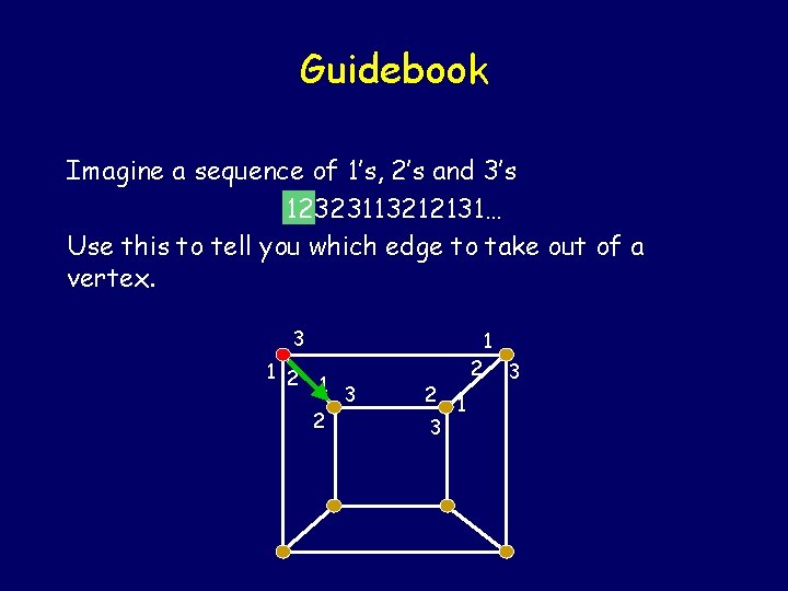
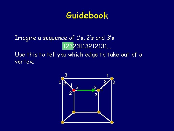
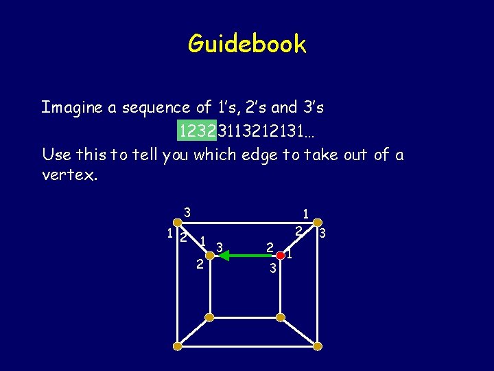
Guidebook Imagine a sequence of 1’s, 2’s and 3’s 12323113212131… Use this to tell you which edge to take out of a vertex. 3 1 2 1 3 2 2 3 2 1 1 3

Guidebook Imagine a sequence of 1’s, 2’s and 3’s 12323113212131… Use this to tell you which edge to take out of a vertex. 3 1 2 1 3 2 2 3 2 1 1 3

Guidebook Imagine a sequence of 1’s, 2’s and 3’s 12323113212131… Use this to tell you which edge to take out of a vertex. 3 1 2 1 3 2 2 3 2 1 1 3

Guidebook Imagine a sequence of 1’s, 2’s and 3’s 12323113212131… Use this to tell you which edge to take out of a vertex. 3 1 2 1 3 2 2 3 2 1 1 3

Universal Guidebooks Theorem: There exists a sequence S such that, for all degree-3 graphs G (with n vertices), and all start vertices, following this sequence will visit all nodes. The length of this sequence S is O(n 3 log n). This is called a “universal traversal sequence”.

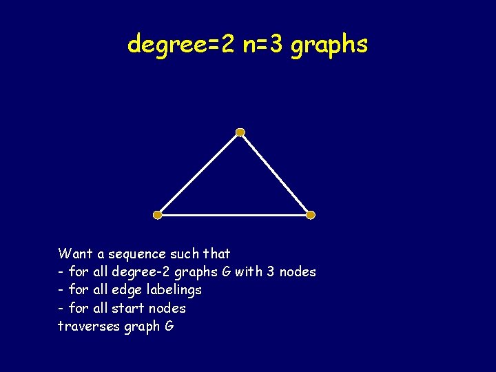
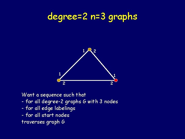
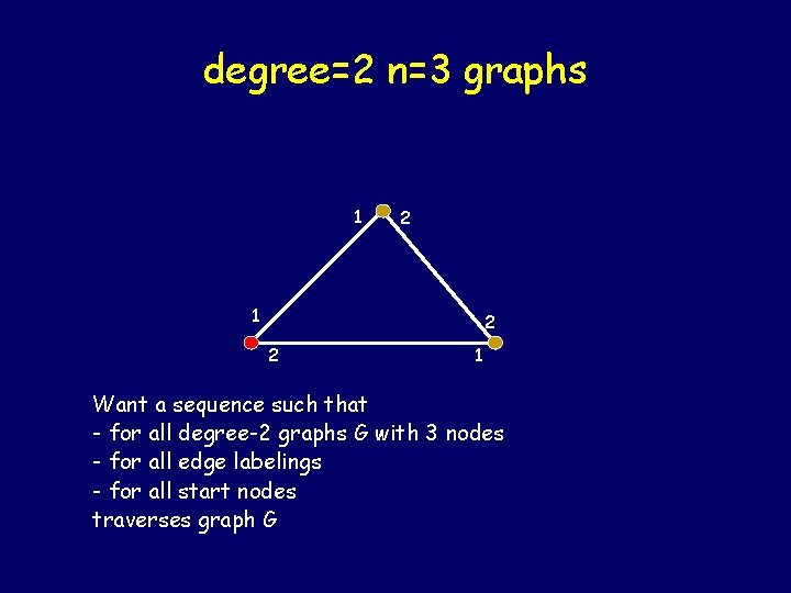
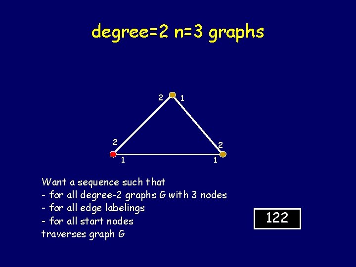
degree=2 n=3 graphs Want a sequence such that - for all degree-2 graphs G with 3 nodes - for all edge labelings - for all start nodes traverses graph G

degree=2 n=3 graphs 1 2 1 1 2 2 Want a sequence such that - for all degree-2 graphs G with 3 nodes - for all edge labelings - for all start nodes traverses graph G

degree=2 n=3 graphs 1 2 2 1 Want a sequence such that - for all degree-2 graphs G with 3 nodes - for all edge labelings - for all start nodes traverses graph G

degree=2 n=3 graphs 2 1 2 2 1 1 Want a sequence such that - for all degree-2 graphs G with 3 nodes - for all edge labelings - for all start nodes traverses graph G 122

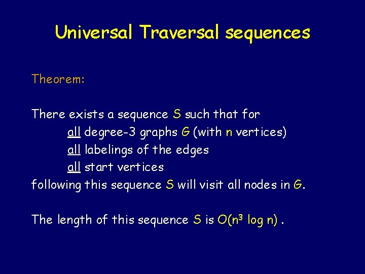
Universal Traversal sequences Theorem: There exists a sequence S such that for all degree-3 graphs G (with n vertices) all labelings of the edges all start vertices following this sequence S will visit all nodes in G. The length of this sequence S is O(n 3 log n).

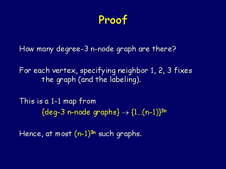
Proof How many degree-3 n-node graph are there? For each vertex, specifying neighbor 1, 2, 3 fixes the graph (and the labeling). This is a 1 -1 map from {deg-3 n-node graphs} {1…(n-1)}3 n Hence, at most (n-1)3 n such graphs.

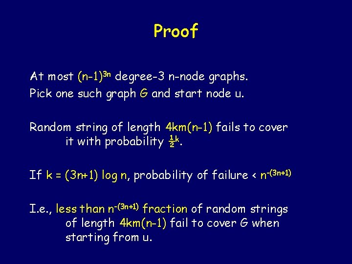
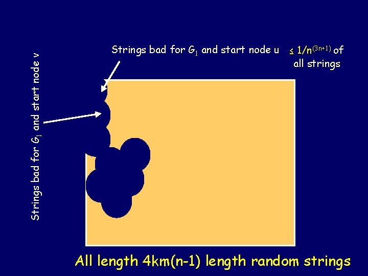
Proof At most (n-1)3 n degree-3 n-node graphs. Pick one such graph G and start node u. Random string of length 4 km(n-1) fails to cover it with probability ½k. If k = (3 n+1) log n, probability of failure < n-(3 n+1) I. e. , less than n-(3 n+1) fraction of random strings of length 4 km(n-1) fail to cover G when starting from u.

Strings bad for G 1 and start node v Strings bad for G 1 and start node u ≤ 1/n(3 n+1) of all strings All length 4 km(n-1) length random strings

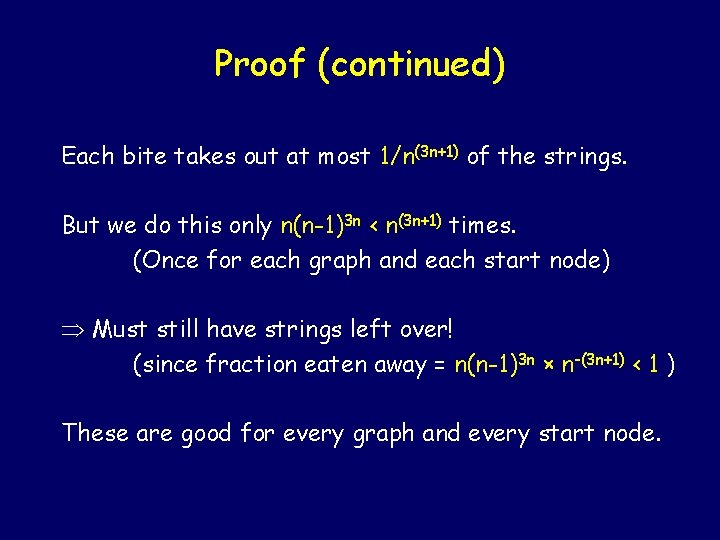
Proof (continued) Each bite takes out at most 1/n(3 n+1) of the strings. But we do this only n(n-1)3 n < n(3 n+1) times. (Once for each graph and each start node) Must still have strings left over! (since fraction eaten away = n(n-1)3 n × n-(3 n+1) < 1 ) These are good for every graph and every start node.

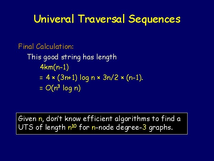
Univeral Traversal Sequences Final Calculation: This good string has length 4 km(n-1) = 4 × (3 n+1) log n × 3 n/2 × (n-1). = O(n 3 log n) Given n, don’t know efficient algorithms to find a UTS of length n 10 for n-node degree-3 graphs.

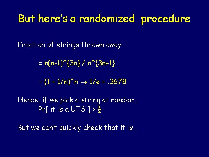
But here’s a randomized procedure Fraction of strings thrown away = n(n-1)^{3 n} / n^{3 n+1} = (1 – 1/n)^n 1/e =. 3678 Hence, if we pick a string at random, Pr[ it is a UTS ] > ½ But we can’t quickly check that it is…

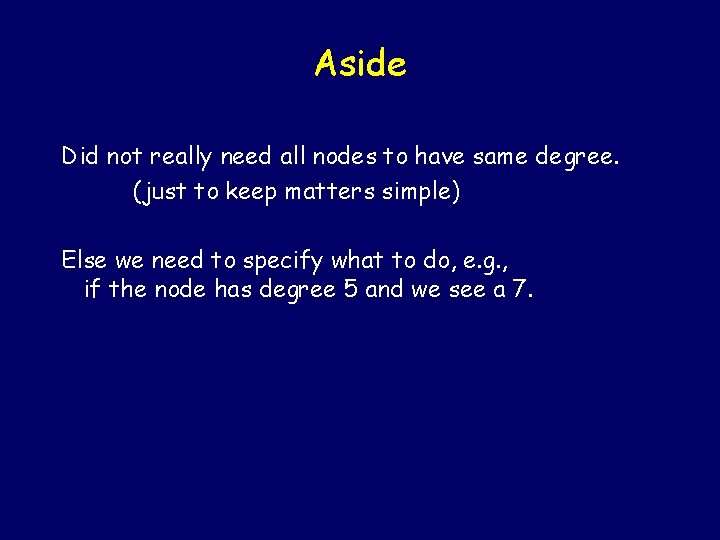
Aside Did not really need all nodes to have same degree. (just to keep matters simple) Else we need to specify what to do, e. g. , if the node has degree 5 and we see a 7.

Cover Time Theorem If the graph G has n nodes and m edges, then the cover time of G is C(G) ≤ 2 m (n – 1)

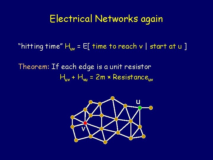
Electrical Networks again “hitting time” Huv = E[ time to reach v | start at u ] Theorem: If each edge is a unit resistor Huv + Hvu = 2 m × Resistanceuv u v -

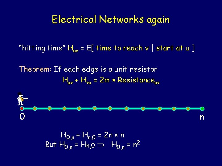
Electrical Networks again “hitting time” Huv = E[ time to reach v | start at u ] Theorem: If each edge is a unit resistor Huv + Hvu = 2 m × Resistanceuv 0 n H 0, n + Hn, 0 = 2 n × n But H 0, n = Hn, 0 H 0, n = n 2

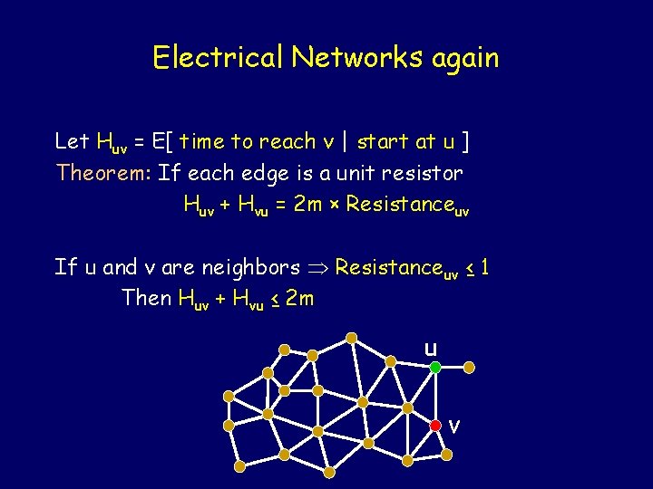
Electrical Networks again Let Huv = E[ time to reach v | start at u ] Theorem: If each edge is a unit resistor Huv + Hvu = 2 m × Resistanceuv If u and v are neighbors Resistanceuv ≤ 1 Then Huv + Hvu ≤ 2 m u -v

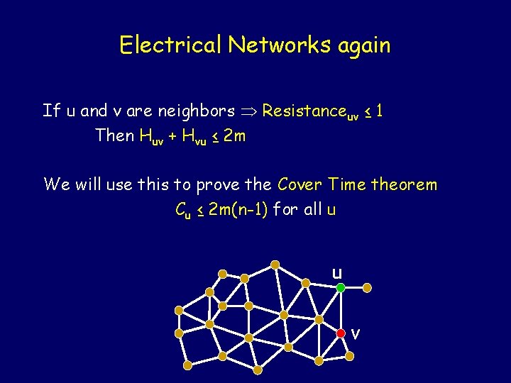
Electrical Networks again If u and v are neighbors Resistanceuv ≤ 1 Then Huv + Hvu ≤ 2 m We will use this to prove the Cover Time theorem Cu ≤ 2 m(n-1) for all u u -v

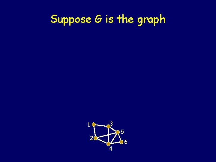
Suppose G is the graph 1 3 5 2 4 6

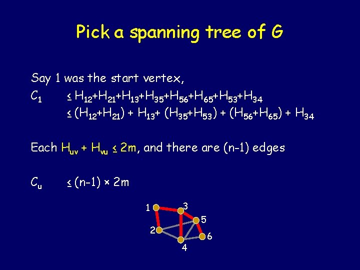
Pick a spanning tree of G Say 1 was the start vertex, C 1 ≤ H 12+H 21+H 13+H 35+H 56+H 65+H 53+H 34 ≤ (H 12+H 21) + H 13+ (H 35+H 53) + (H 56+H 65) + H 34 Each Huv + Hvu ≤ 2 m, and there are (n-1) edges Cu ≤ (n-1) × 2 m 1 3 2 4 -5 6

Cover Time Theorem If the graph G has n nodes and m edges, then the cover time of G is C(G) ≤ 2 m (n – 1)

Random walks on infinite graphs

A drunk man will find his way home, but a drunk bird may get lost forever - Shizuo Kakutani

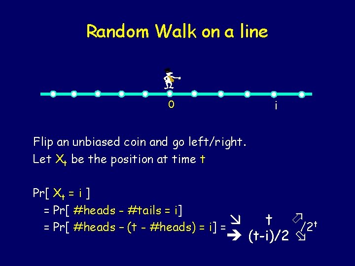
Random Walk on a line i 0 Flip an unbiased coin and go left/right. Let Xt be the position at time t Pr[ Xt = i ] = Pr[ #heads - #tails = i] = Pr[ #heads – (t - #heads) = i] = t /2 t (t-i)/2

Unbiased Random Walk 0 2 t Pr[ X 2 t = 0 ] = /22 t t Stirling’s approximation: n! = Θ((n/e)n × √n) p n 2 £ ( ( 2 en ) 2 n ) p Hence: (2 n)!/(n!)2 = n £ (( e )n n ) = Θ(22 n/n½)

Unbiased Random Walk 0 2 t Pr[ X 2 t = 0 ] = /22 t ≤ Θ(1/√t) t Y 2 t = indicator for (X 2 t = 0) Sterling’s approx. E[ Y 2 t ] = Θ(1/√t) Z 2 n = number of visits to origin in 2 n steps. E[ Z 2 n ] = E[ t = 1…n Y 2 t ] = Θ(1/√ 1 + 1/√ 2 +…+ 1/√n) = Θ(√n)

In n steps, you expect to return to the origin Θ(√n) times!

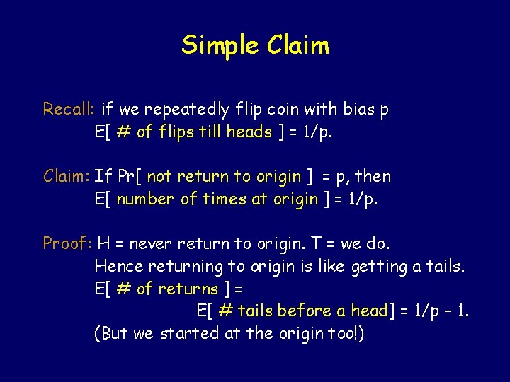
Simple Claim Recall: if we repeatedly flip coin with bias p E[ # of flips till heads ] = 1/p. Claim: If Pr[ not return to origin ] = p, then E[ number of times at origin ] = 1/p. Proof: H = never return to origin. T = we do. Hence returning to origin is like getting a tails. E[ # of returns ] = E[ # tails before a head] = 1/p – 1. (But we started at the origin too!)

We will return… Claim: If Pr[ not return to origin ] = p, then E[ number of times at origin ] = 1/p. Theorem: Pr[ we return to origin ] = 1. Proof: Suppose not. Hence p = Pr[ never return ] > 0. E [ #times at origin ] = 1/p = constant. But we showed that E[ Zn ] = Θ(√n) ∞

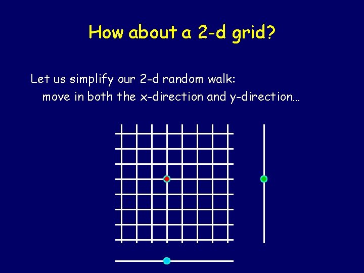
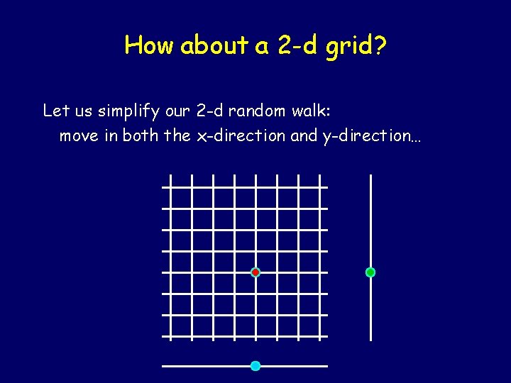
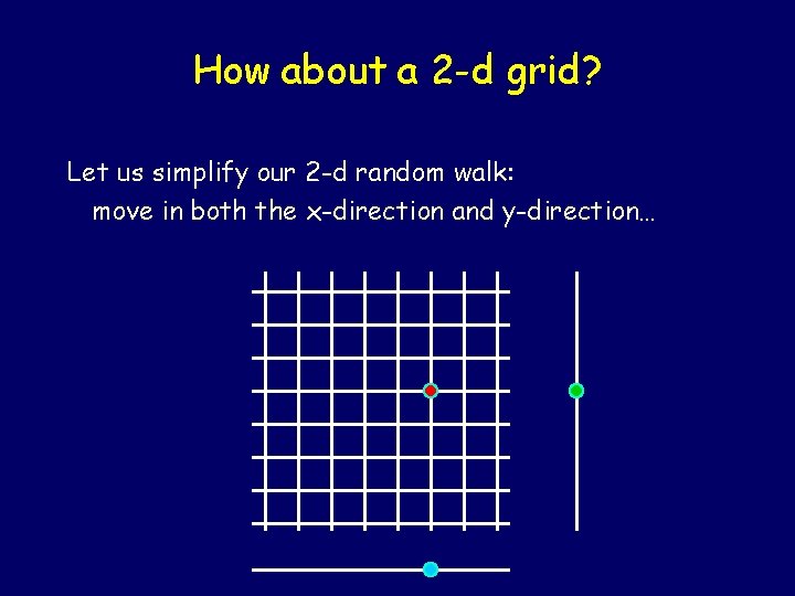
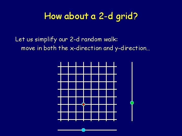
How about a 2 -d grid? Let us simplify our 2 -d random walk: move in both the x-direction and y-direction…

How about a 2 -d grid? Let us simplify our 2 -d random walk: move in both the x-direction and y-direction…

How about a 2 -d grid? Let us simplify our 2 -d random walk: move in both the x-direction and y-direction…

How about a 2 -d grid? Let us simplify our 2 -d random walk: move in both the x-direction and y-direction…

How about a 2 -d grid? Let us simplify our 2 -d random walk: move in both the x-direction and y-direction…

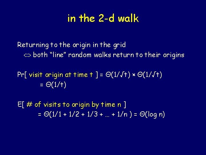
in the 2 -d walk Returning to the origin in the grid both “line” random walks return to their origins Pr[ visit origin at time t ] = Θ(1/√t) × Θ(1/√t) = Θ(1/t) E[ # of visits to origin by time n ] = Θ(1/1 + 1/2 + 1/3 + … + 1/n ) = Θ(log n)

We will return (again!)… Claim: If Pr[ not return to origin ] = p, then E[ number of times at origin ] = 1/p. Theorem: Pr[ we return to origin ] = 1. Proof: Suppose not. Hence p = Pr[ never return ] > 0. E [ #times at origin ] = 1/p = constant. But we showed that E[ Zn ] = Θ(log n) ∞

But in 3 -d Pr[ visit origin at time t ] = Θ(1/√t)3 = Θ(1/t 3/2) limn ∞ E[ # of visits by time n ] < K (constant) Hence Pr[ never return to origin ] > 1/K.