T tests ANOVAs and regression Tom Jenkins Ellen

T tests, ANOVAs and regression Tom Jenkins Ellen Meierotto SPM Methods for Dummies 2007

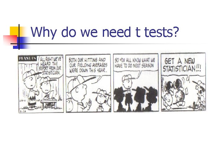
Why do we need t tests?

Objectives n n n Types of error Probability distribution Z scores T tests ANOVAs

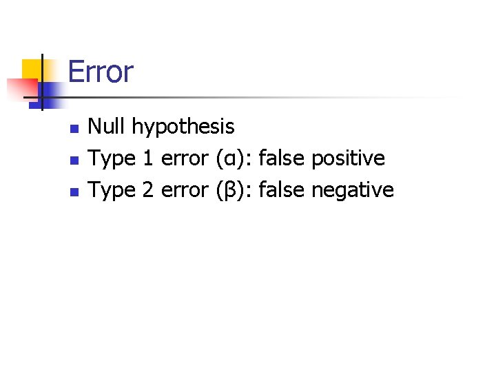
Error n n n Null hypothesis Type 1 error (α): false positive Type 2 error (β): false negative

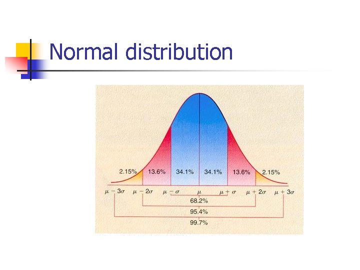
Normal distribution

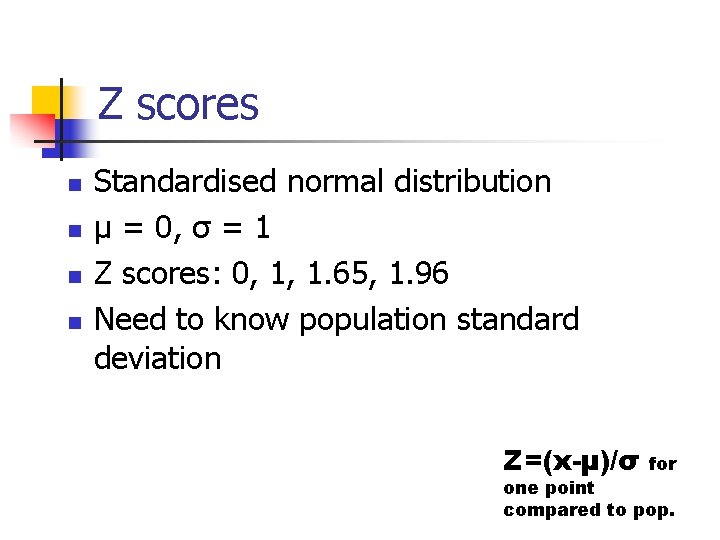
Z scores n n Standardised normal distribution µ = 0, σ = 1 Z scores: 0, 1, 1. 65, 1. 96 Need to know population standard deviation Z=(x-μ)/σ for one point compared to pop.

T tests n n Comparing means 1 sample t 2 sample t Paired t

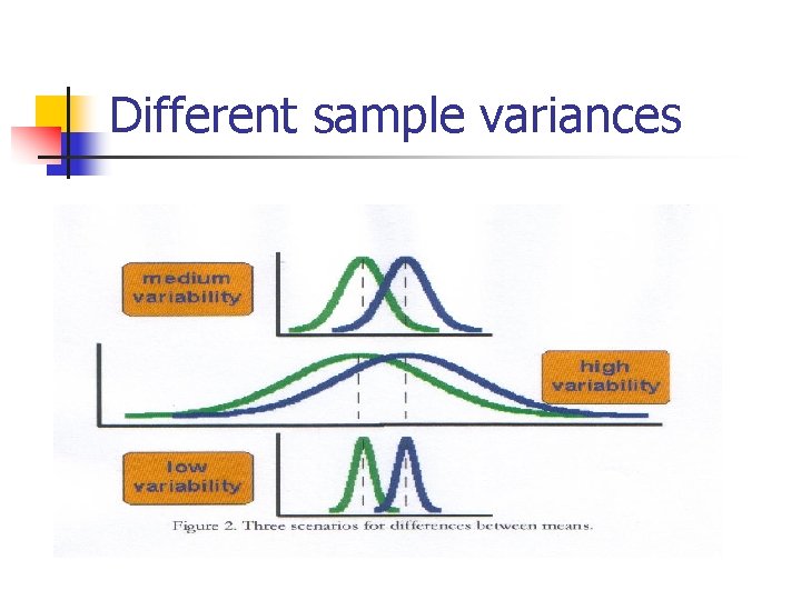
Different sample variances

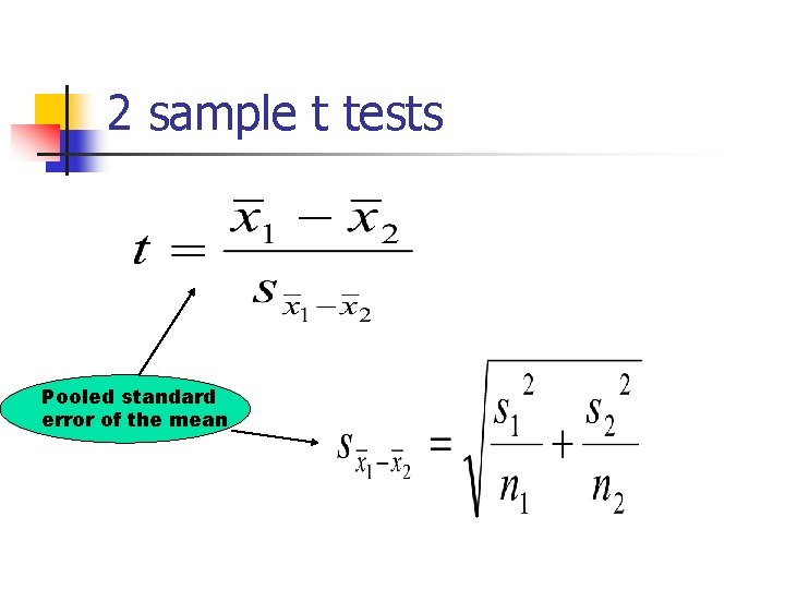
2 sample t tests Pooled standard error of the mean

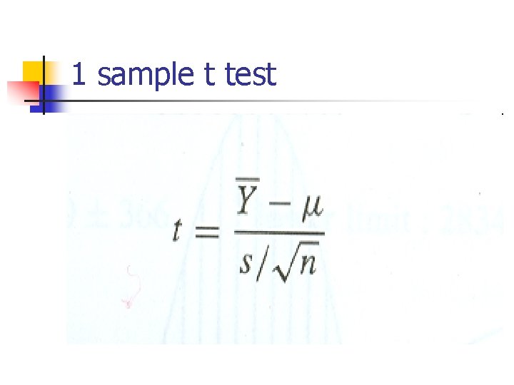
1 sample t test

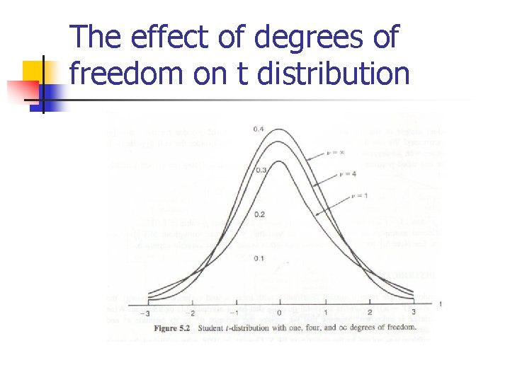
The effect of degrees of freedom on t distribution

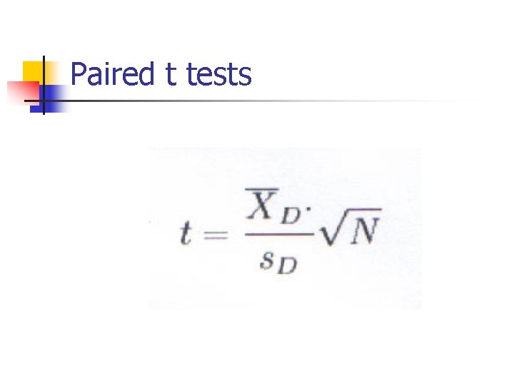
Paired t tests

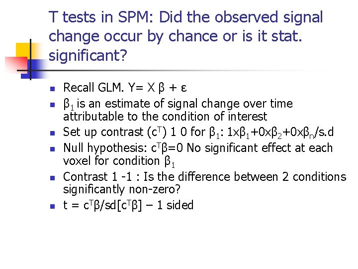
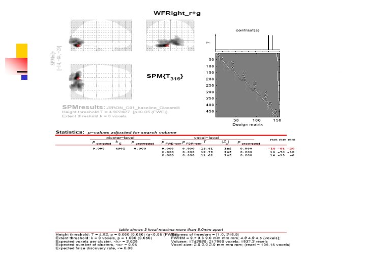
T tests in SPM: Did the observed signal change occur by chance or is it stat. significant? n n n Recall GLM. Y= X β + ε β 1 is an estimate of signal change over time attributable to the condition of interest Set up contrast (c. T) 1 0 for β 1: 1 xβ 1+0 xβ 2+0 xβn/s. d Null hypothesis: c. Tβ=0 No significant effect at each voxel for condition β 1 Contrast 1 -1 : Is the difference between 2 conditions significantly non-zero? t = c. Tβ/sd[c. Tβ] – 1 sided

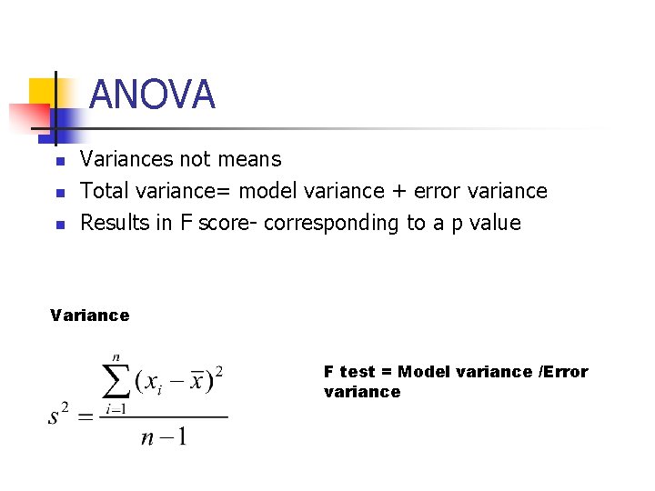
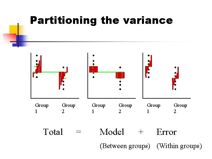
ANOVA n n n Variances not means Total variance= model variance + error variance Results in F score- corresponding to a p value Variance F test = Model variance /Error variance

Partitioning the variance Group 1 Group 2 Total = Group 1 Group 2 Model + Group 2 Error (Between groups) (Within groups)

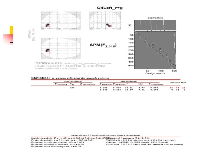
T vs F tests n n F tests- any differences between multiple groups, interactions Have to determine where differences are post-hoc SPM- T- one tailed (con) SPM- F- two tailed (ess)

Conclusions n n T tests describe how unlikely it is that experimental differences are due to chance Higher the t score, smaller the p value, more unlikely to be due to chance Can compare sample with population or 2 samples, paired or unpaired ANOVA/F tests are similar but use variances instead of means and can be applied to more than 2 groups and other more complex scenarios

Acknowledgements n n Mf. D slides 2004 -2006 Van Belle, Biostatistics Human Brain Function Wikipedia

Correlation and Regression

Topics Covered: n n Is there a relationship between x and y? What is the strength of this relationship n n Can we describe this relationship and use it to predict y from x? n n Regression Is the relationship we have described statistically significant? n n Pearson’s r F- and t-tests Relevance to SPM n GLM

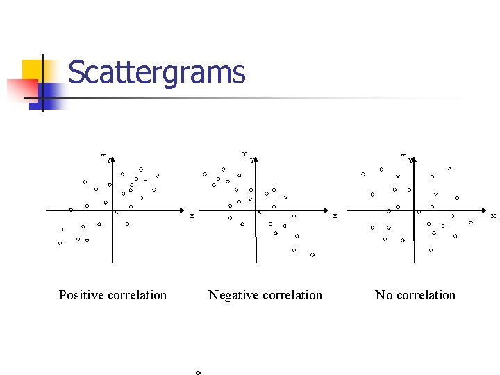
Relationship between x and y n n n Correlation describes the strength and direction of a linear relationship between two variables Regression tells you how well a certain independent variable predicts a dependent variable CORRELATION CAUSATION n In order to infer causality: manipulate independent variable and observe effect on dependent variable

Scattergrams Y Y Y X Positive correlation Y Y Y X X Negative correlation No correlation

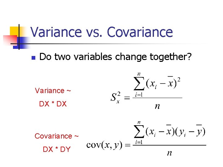
Variance vs. Covariance n Do two variables change together? Variance ~ DX * DX Covariance ~ DX * DY

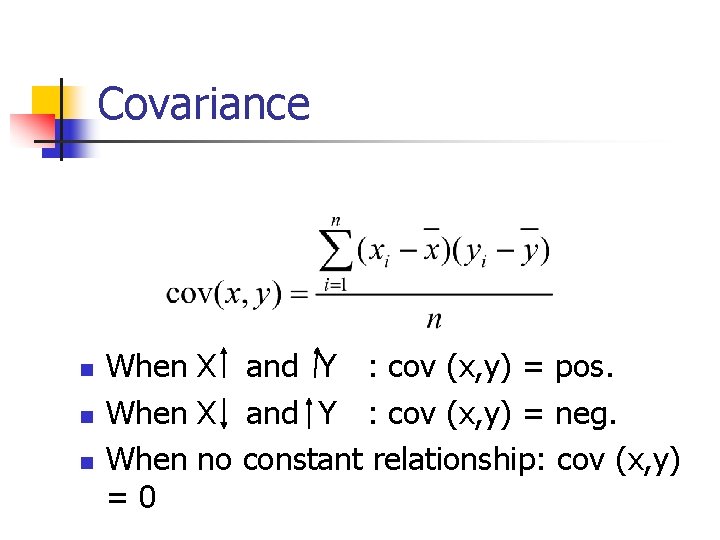
Covariance n n n When X and Y : cov (x, y) = pos. When X and Y : cov (x, y) = neg. When no constant relationship: cov (x, y) = 0

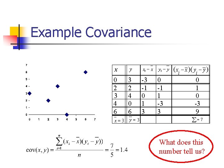
Example Covariance x y xi - x yi - y 0 2 3 4 6 3 2 4 0 6 -3 -1 0 1 3 0 -1 1 -3 3 x=3 y=3 ( xi - x )( yi - y ) 0 1 0 -3 9 å= 7 What does this number tell us?

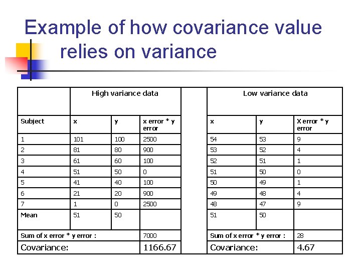
Example of how covariance value relies on variance High variance data Subject x y x error * y error 1 100 2500 2 81 80 900 3 61 60 4 51 5 Low variance data x y X error * y error 54 53 9 53 52 4 100 52 51 1 50 0 51 50 0 41 40 100 50 49 1 6 21 20 900 49 48 4 7 1 0 2500 48 47 9 Mean 51 50 Sum of x error * y error : 7000 Sum of x error * y error : 28 Covariance: 1166. 67 Covariance: 4. 67

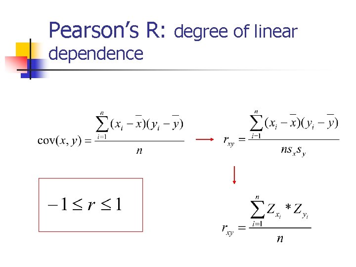
Pearson’s R n Covariance does not really tell us anything n n Solution: standardise this measure Pearson’s R: standardise by adding std to equation:

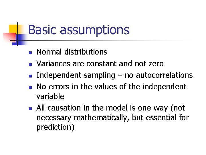
Basic assumptions n n n Normal distributions Variances are constant and not zero Independent sampling – no autocorrelations No errors in the values of the independent variable All causation in the model is one-way (not necessary mathematically, but essential for prediction)

Pearson’s R: degree of linear dependence

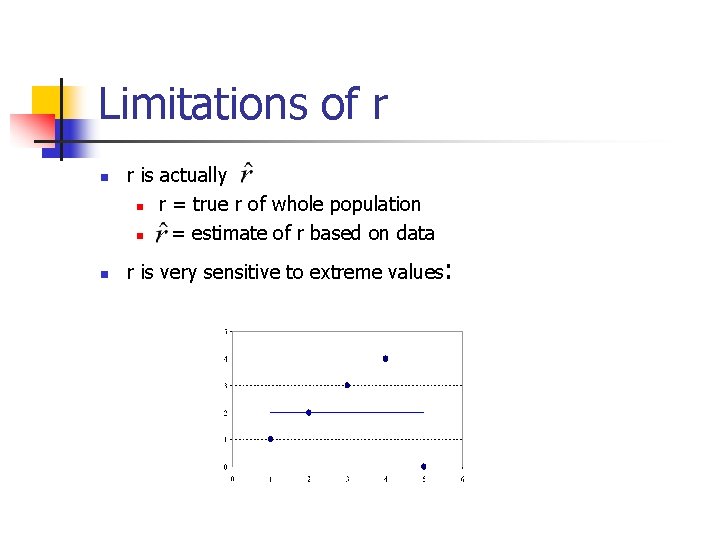
Limitations of r n n r is actually n r = true r of whole population n = estimate of r based on data r is very sensitive to extreme values:

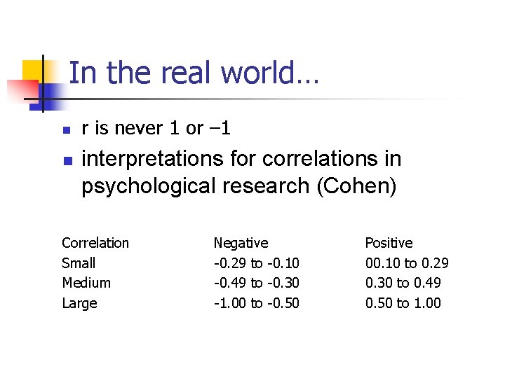
In the real world… n n r is never 1 or – 1 interpretations for correlations in psychological research (Cohen) Correlation Small Medium Large Negative -0. 29 to -0. 10 -0. 49 to -0. 30 -1. 00 to -0. 50 Positive 00. 10 to 0. 29 0. 30 to 0. 49 0. 50 to 1. 00

Regression n n Correlation tells you if there is an association between x and y but it doesn’t describe the relationship or allow you to predict one variable from the other. To do this we need REGRESSION!

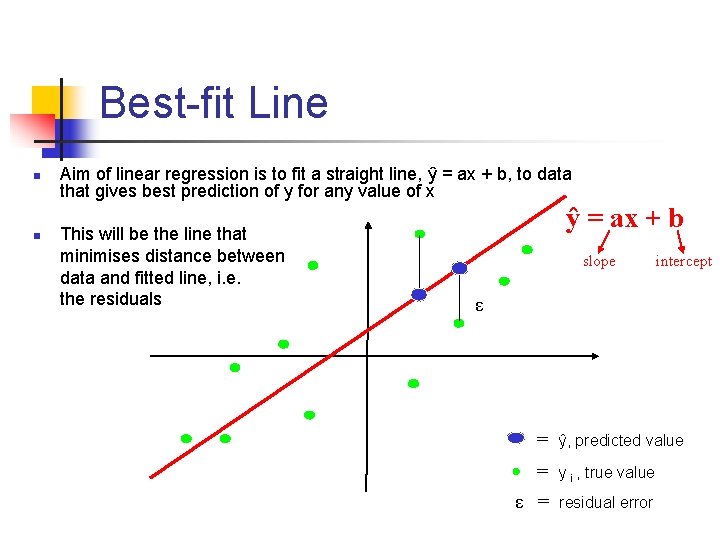
Best-fit Line n n Aim of linear regression is to fit a straight line, ŷ = ax + b, to data that gives best prediction of y for any value of x This will be the line that minimises distance between data and fitted line, i. e. the residuals ŷ = ax + b slope intercept ε = ŷ, predicted value = y i , true value ε = residual error

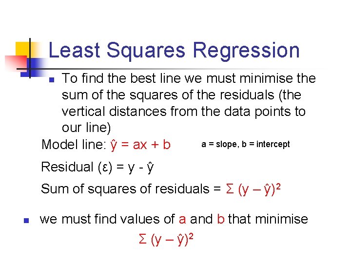
Least Squares Regression To find the best line we must minimise the sum of the squares of the residuals (the vertical distances from the data points to our line) a = slope, b = intercept Model line: ŷ = ax + b n Residual (ε) = y - ŷ Sum of squares of residuals = Σ (y – ŷ)2 n we must find values of a and b that minimise Σ (y – ŷ)2

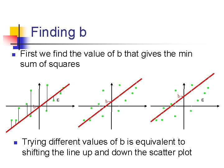
Finding b n First we find the value of b that gives the min sum of squares ε b n b b Trying different values of b is equivalent to shifting the line up and down the scatter plot ε

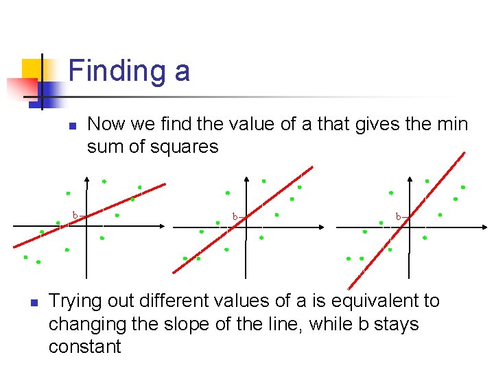
Finding a n b n Now we find the value of a that gives the min sum of squares b b Trying out different values of a is equivalent to changing the slope of the line, while b stays constant

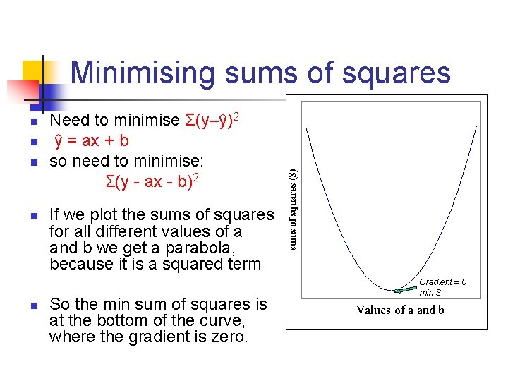
n n n Need to minimise Σ(y–ŷ)2 ŷ = ax + b so need to minimise: Σ(y - ax - b)2 If we plot the sums of squares for all different values of a and b we get a parabola, because it is a squared term So the min sum of squares is at the bottom of the curve, where the gradient is zero. sums of squares (S) Minimising sums of squares Gradient = 0 min S Values of a and b

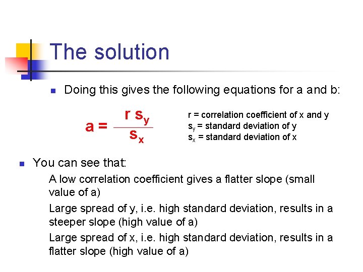
The maths bit n n So we can find a and b that give min sum of squares by taking partial derivatives of Σ(y ax - b)2 with respect to a and b separately Then we solve these for 0 to give us the values of a and b that give the min sum of squares

The solution n Doing this gives the following equations for a and b: r sy a= s x n r = correlation coefficient of x and y sy = standard deviation of y sx = standard deviation of x You can see that: § § § A low correlation coefficient gives a flatter slope (small value of a) Large spread of y, i. e. high standard deviation, results in a steeper slope (high value of a) Large spread of x, i. e. high standard deviation, results in a flatter slope (high value of a)

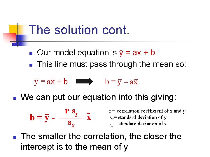
The solution cont. n n Our model equation is ŷ = ax + b This line must pass through the mean so: y = ax + b n We can put our equation into this giving: b=yn b = y – ax r sy x sx r = correlation coefficient of x and y sy = standard deviation of y sx = standard deviation of x The smaller the correlation, the closer the intercept is to the mean of y

Back to the model n We can calculate the regression line for any data, but the important question is: How well does this line fit the data, or how good is it at predicting y from x?

How good is our model? n n Total variance of y: sy 2 = n-1 = SSy dfy Variance of predicted y values (ŷ): sŷ 2 = n ∑(y – y)2 ∑(ŷ – y)2 n-1 = SSpred dfŷ Error variance: serror 2 = ∑(y – ŷ)2 n-2 = SSer dfer This is the variance explained by our regression model This is the variance of the error between our predicted y values and the actual y values, and thus is the variance in y that is NOT explained by the regression model

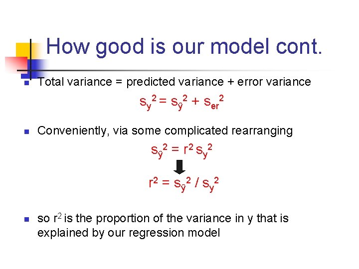
How good is our model cont. n Total variance = predicted variance + error variance sy 2 = sŷ 2 + ser 2 n Conveniently, via some complicated rearranging sŷ 2 = r 2 sy 2 r 2 = sŷ 2 / sy 2 n so r 2 is the proportion of the variance in y that is explained by our regression model

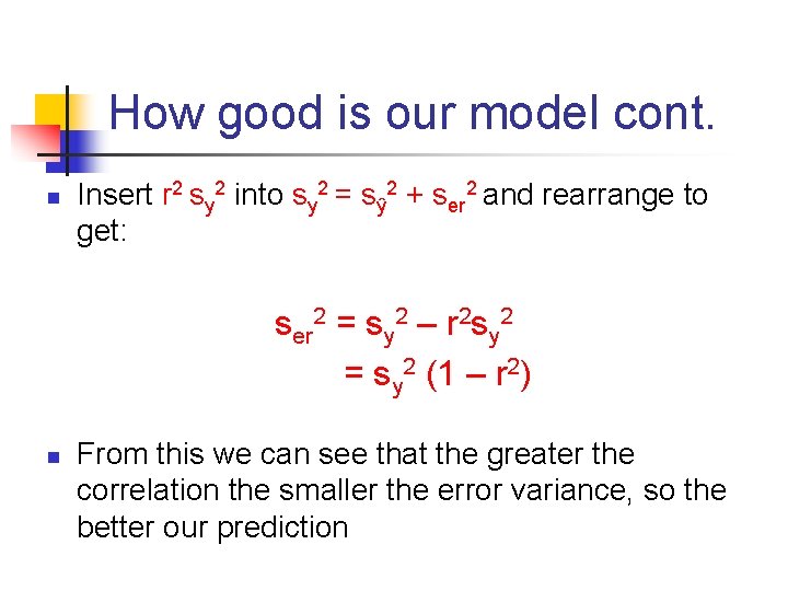
How good is our model cont. n Insert r 2 sy 2 into sy 2 = sŷ 2 + ser 2 and rearrange to get: ser 2 = sy 2 – r 2 sy 2 = sy 2 (1 – r 2) n From this we can see that the greater the correlation the smaller the error variance, so the better our prediction

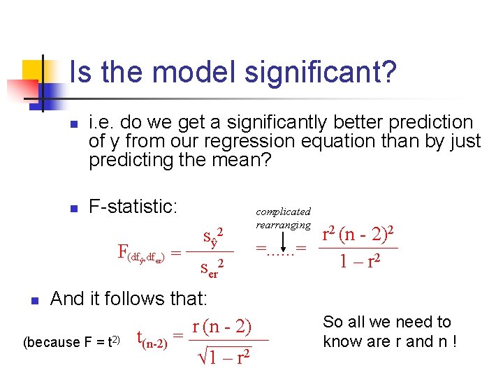
Is the model significant? n n i. e. do we get a significantly better prediction of y from our regression equation than by just predicting the mean? F-statistic: F(df , df ) = ŷ er sŷ 2 ser 2 And it follows that: r (n - 2) 2) t = (because F = t (n-2) √ 1 – r 2 complicated rearranging r 2 (n - 2)2 =. . . = 1 – r 2 n So all we need to know are r and n !

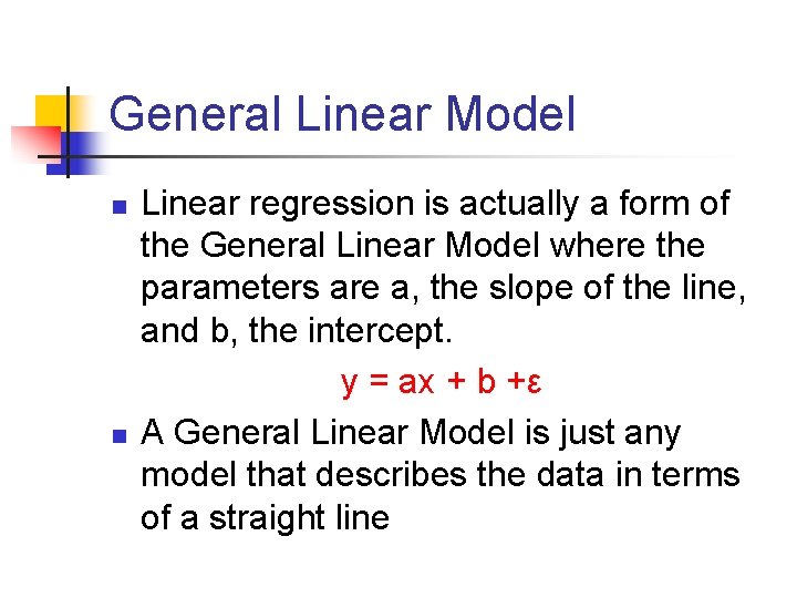
General Linear Model n n Linear regression is actually a form of the General Linear Model where the parameters are a, the slope of the line, and b, the intercept. y = ax + b +ε A General Linear Model is just any model that describes the data in terms of a straight line

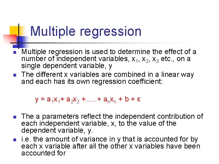
Multiple regression n n Multiple regression is used to determine the effect of a number of independent variables, x 1, x 2, x 3 etc. , on a single dependent variable, y The different x variables are combined in a linear way and each has its own regression coefficient: y = a 1 x 1+ a 2 x 2 +…. . + anxn + b + ε n n The a parameters reflect the independent contribution of each independent variable, x, to the value of the dependent variable, y. i. e. the amount of variance in y that is accounted for by each x variable after all the other x variables have been accounted for

SPM n n n Linear regression is a GLM that models the effect of one independent variable, x, on ONE dependent variable, y Multiple Regression models the effect of several independent variables, x 1, x 2 etc, on ONE dependent variable, y Both are types of General Linear Model GLM can also allow you to analyse the effects of several independent x variables on several dependent variables, y 1, y 2, y 3 etc, in a linear combination This is what SPM does and will be explained soon…