SYDE 575 Digital Image Processing Using Discrete Gradients

SYDE 575: Digital Image Processing Using Discrete Gradients: Edge Detection & Edge Enhancement/Sharpening Exact Blur Compensation Textbook 10. 2. 5 (edge detection), 3. 6 (sharpening), blackboard (exact blur compensation – review ztransform on your own)

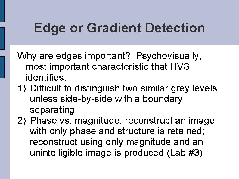
Edge or Gradient Detection Why are edges important? Psychovisually, most important characteristic that HVS identifies. 1) Difficult to distinguish two similar grey levels unless side-by-side with a boundary separating 2) Phase vs. magnitude: reconstruct an image with only phase and structure is retained; reconstruct using only magnitude and an unintelligible image is produced (Lab #3)

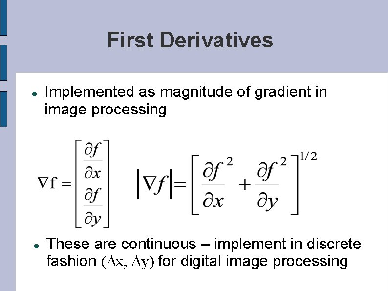
First Derivatives Implemented as magnitude of gradient in image processing These are continuous – implement in discrete fashion (Dx, Dy) for digital image processing

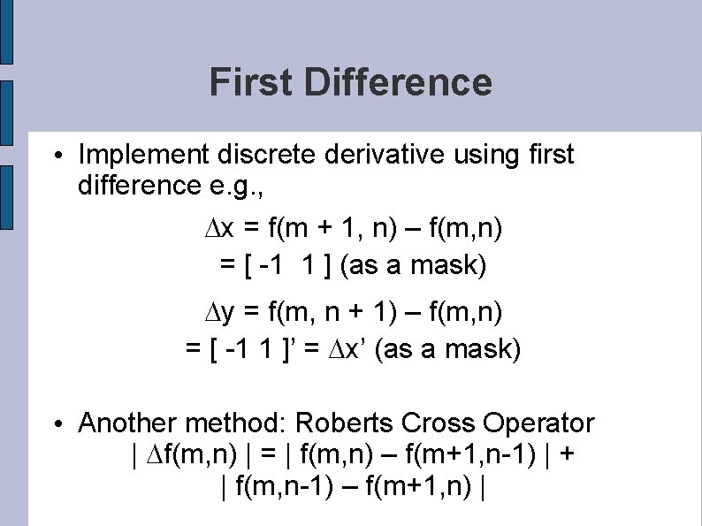
First Difference • Implement discrete derivative using first difference e. g. , Dx = f(m + 1, n) – f(m, n) = [ -1 1 ] (as a mask) Dy = f(m, n + 1) – f(m, n) = [ -1 1 ]’ = Dx’ (as a mask) • Another method: Roberts Cross Operator | Df(m, n) | = | f(m, n) – f(m+1, n-1) | + | f(m, n-1) – f(m+1, n) |

First Difference • First difference operators are not effective • Very sensitive to noise because of small spatial extent • Solution: use a larger mask

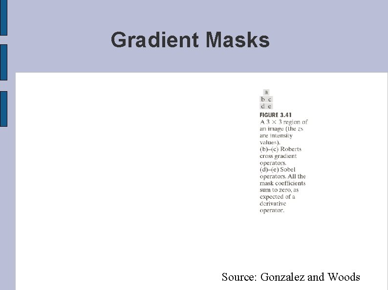
Gradient Masks Source: Gonzalez and Woods

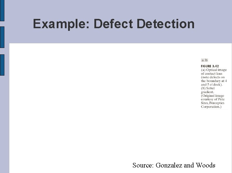
Example: Defect Detection Source: Gonzalez and Woods

1 -D Example

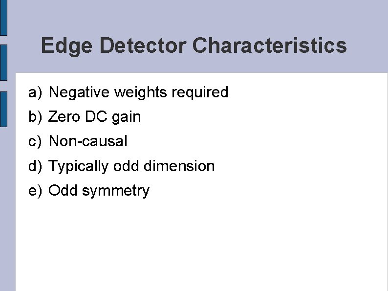
Edge Detector Characteristics a) Negative weights required b) Zero DC gain c) Non-causal d) Typically odd dimension e) Odd symmetry

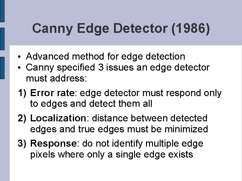
Canny Edge Detector (1986) • Advanced method for edge detection • Canny specified 3 issues an edge detector must address: 1) Error rate: edge detector must respond only to edges and detect them all 2) Localization: distance between detected edges and true edges must be minimized 3) Response: do not identify multiple edge pixels where only a single edge exists

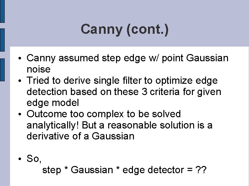
Canny (cont. ) • Canny assumed step edge w/ point Gaussian noise • Tried to derive single filter to optimize edge detection based on these 3 criteria for given edge model • Outcome too complex to be solved analytically! But a reasonable solution is a derivative of a Gaussian • So, step * Gaussian * edge detector = ? ?

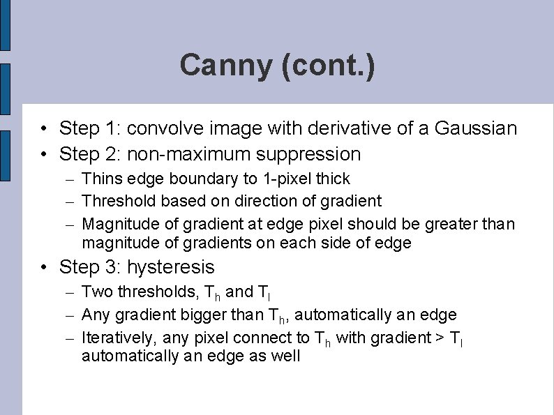
Canny (cont. ) • Step 1: convolve image with derivative of a Gaussian • Step 2: non-maximum suppression – Thins edge boundary to 1 -pixel thick – Threshold based on direction of gradient – Magnitude of gradient at edge pixel should be greater than magnitude of gradients on each side of edge • Step 3: hysteresis – Two thresholds, Th and Tl – Any gradient bigger than Th, automatically an edge – Iteratively, any pixel connect to Th with gradient > Tl automatically an edge as well

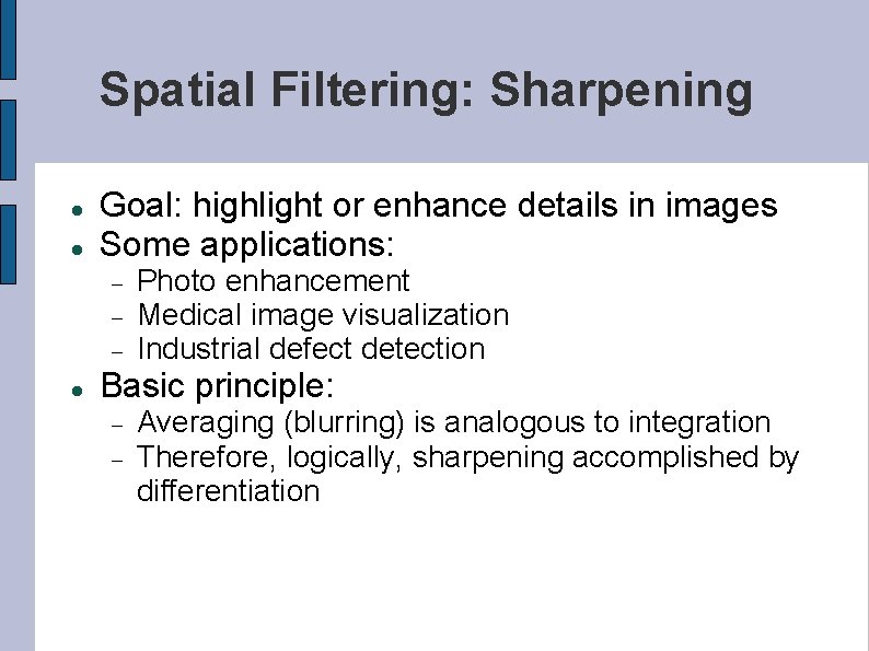
Spatial Filtering: Sharpening Goal: highlight or enhance details in images Some applications: Photo enhancement Medical image visualization Industrial defect detection Basic principle: Averaging (blurring) is analogous to integration Therefore, logically, sharpening accomplished by differentiation

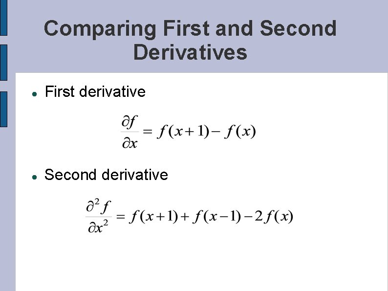
Comparing First and Second Derivatives First derivative Second derivative

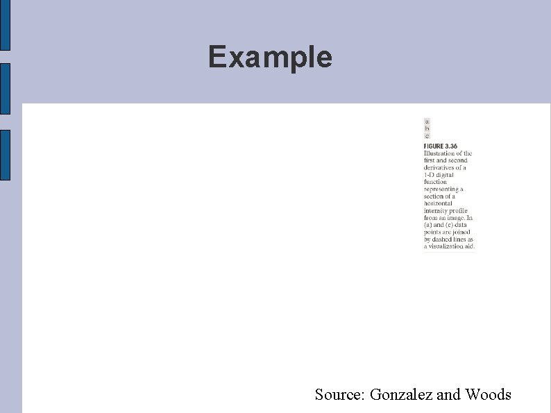
Derivatives of Digital Function Second-order derivatives have stronger response to fine detail (e. g. , thin lines and points) Second-order derivatives have a non-zero response to ramps First-order derivatives have stronger response to step changes Second-order derivatives produce double response at step changes

Example Source: Gonzalez and Woods

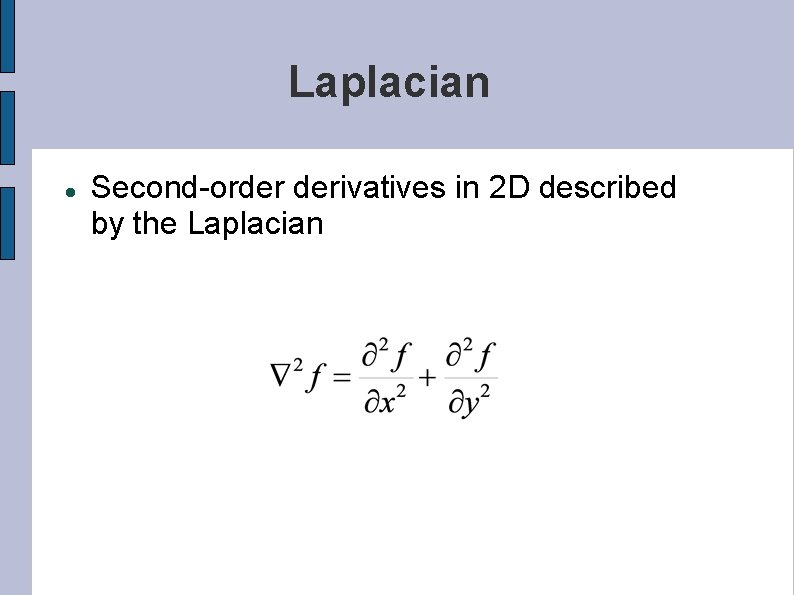
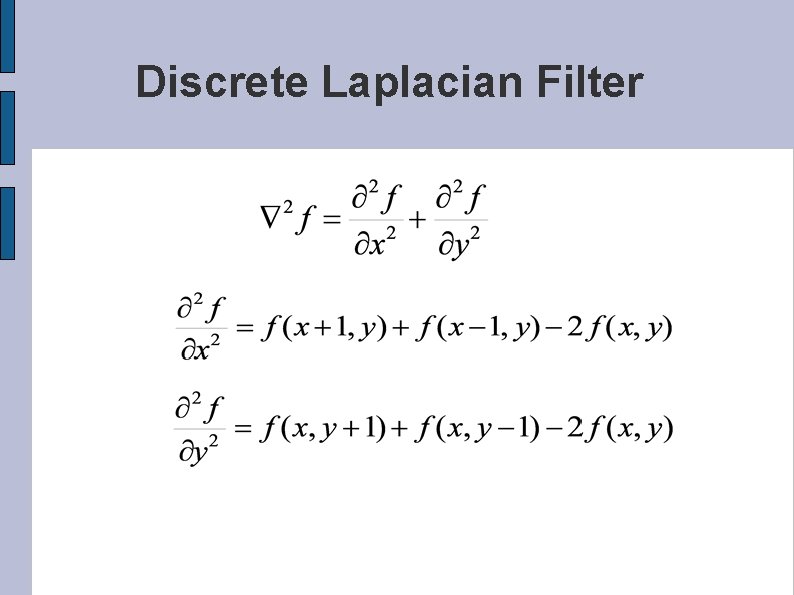
Laplacian Second-order derivatives in 2 D described by the Laplacian

Discrete Laplacian Filter

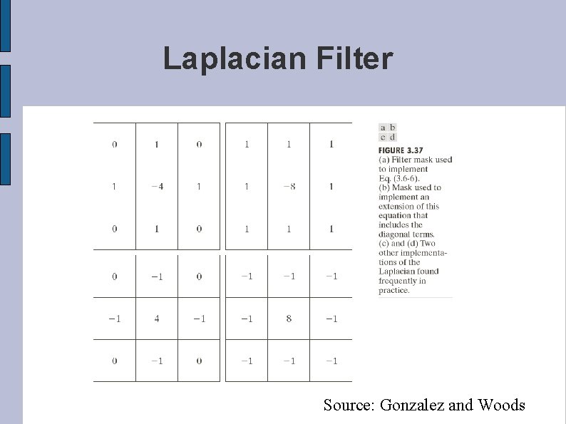
Laplacian Filter Source: Gonzalez and Woods

1 – Laplacian in Practice • How can the second derivative (Laplacian) be used?

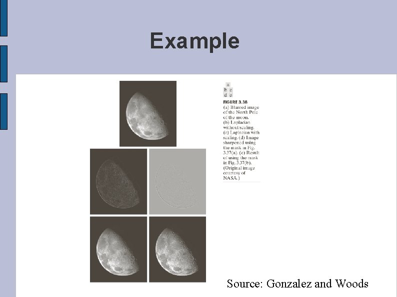
Example Source: Gonzalez and Woods

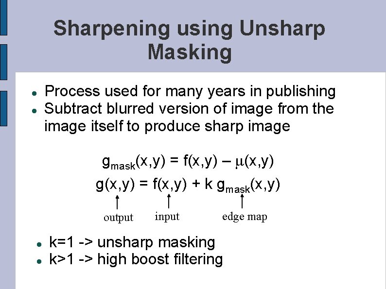
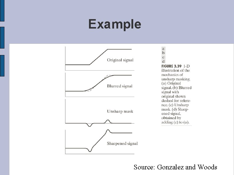
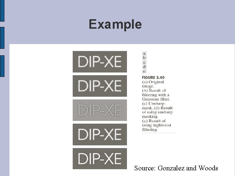
Sharpening using Unsharp Masking Process used for many years in publishing Subtract blurred version of image from the image itself to produce sharp image gmask(x, y) = f(x, y) – m(x, y) g(x, y) = f(x, y) + k gmask(x, y) output input edge map k=1 -> unsharp masking k>1 -> high boost filtering

Example Source: Gonzalez and Woods

Impulse Response for Unsharp Masking

Example Source: Gonzalez and Woods

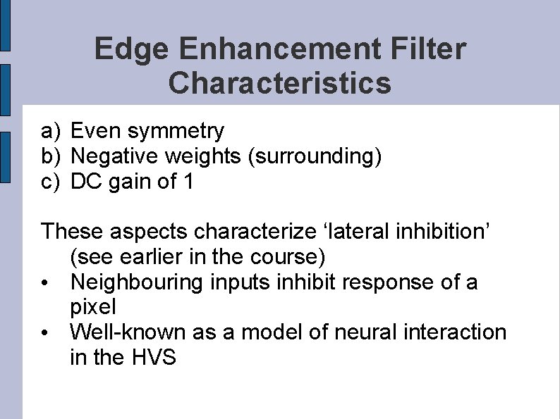
Edge Enhancement Filter Characteristics a) Even symmetry b) Negative weights (surrounding) c) DC gain of 1 These aspects characterize ‘lateral inhibition’ (see earlier in the course) • Neighbouring inputs inhibit response of a pixel • Well-known as a model of neural interaction in the HVS

Exact Blur Compensation • Use of complex number to solve difference equation representing inverse system • Use of z-transform for solving inverse system for general blur model • Blackboard notes