SYDE 575 Introduction to Image Processing Image Enhancement

SYDE 575: Introduction to Image Processing Image Enhancement by Smoothing Textbook Sections 3. 4 – 3. 5, 5. 3. 1 -5. 3. 2

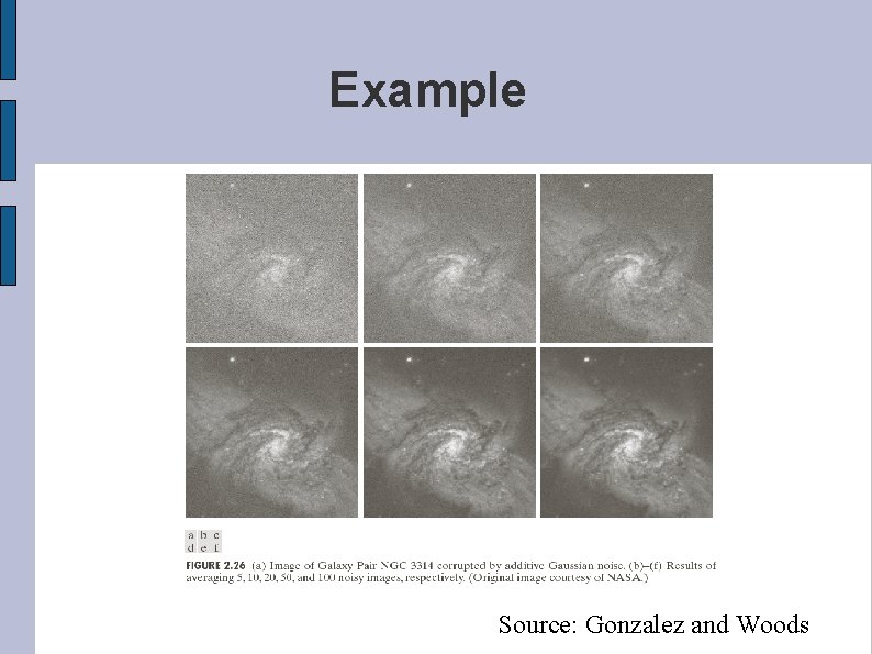
Noise Reduction by Image Averaging We want to be able to reduce the amount of noise in an image Assume that the noise process has a mean of zero One approach is to take many images f(x, y) of the same scene and use these to generate a noise-free image g(x, y)

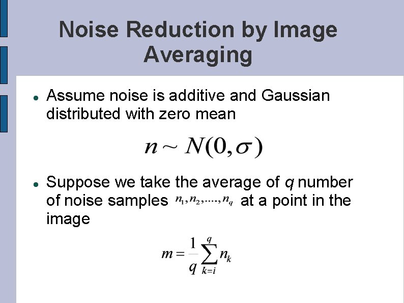
Noise Reduction by Image Averaging Assume noise is additive and Gaussian distributed with zero mean Suppose we take the average of q number of noise samples at a point in the image

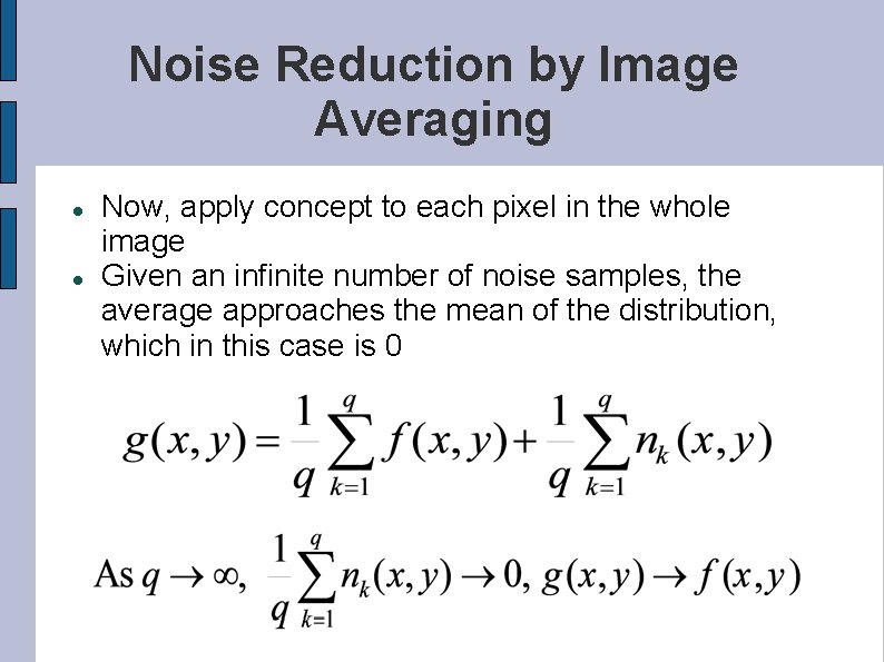
Noise Reduction by Image Averaging Now, apply concept to each pixel in the whole image Given an infinite number of noise samples, the average approaches the mean of the distribution, which in this case is 0

Example Source: Gonzalez and Woods

Noise Reduction by Spatial Filtering Image averaging takes advantage of information redundancy from the individual images to reduce noise Not always possible to acquire so many images! Images may not be perfectly registered so errors due to spatial misalignment Alternative option: Take advantage of information redundancy from different pixels within the same image to reduce noise

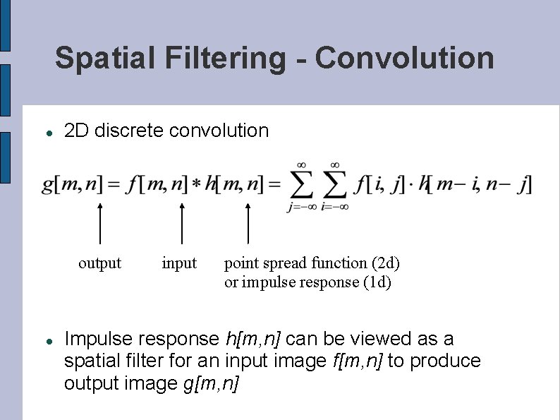
Spatial Filtering - Convolution 2 D discrete convolution output input point spread function (2 d) or impulse response (1 d) Impulse response h[m, n] can be viewed as a spatial filter for an input image f[m, n] to produce output image g[m, n]

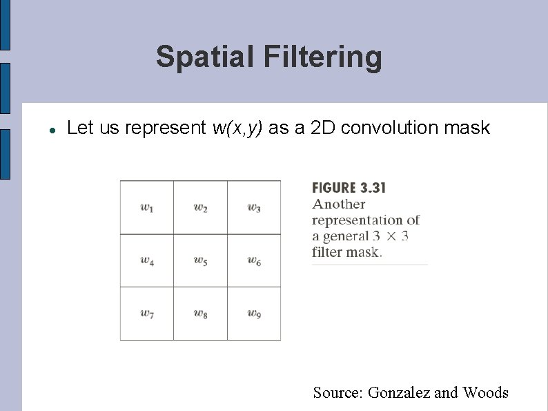
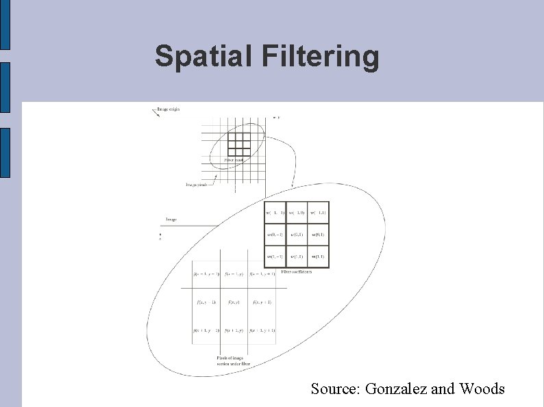
Spatial Filtering Let us represent w(x, y) as a 2 D convolution mask Source: Gonzalez and Woods

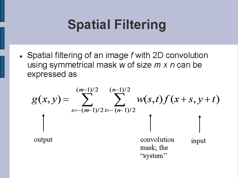
Spatial Filtering Spatial filtering of an image f with 2 D convolution using symmetrical mask w of size m x n can be expressed as output convolution mask; the “system” input

Spatial Filtering Source: Gonzalez and Woods

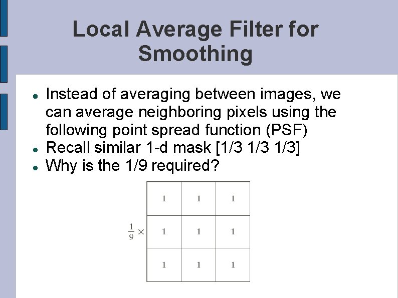
Local Average Filter for Smoothing Instead of averaging between images, we can average neighboring pixels using the following point spread function (PSF) Recall similar 1 -d mask [1/3 1/3] Why is the 1/9 required?

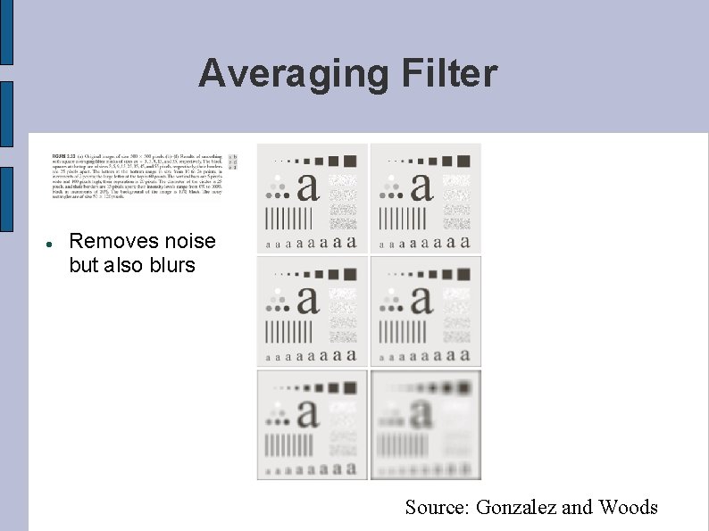
Averaging Filter Removes noise but also blurs Source: Gonzalez and Woods

Properties of Averaging Filter • • • Linear? Shift Invariant? Memory? Causal? Stable? Invertible?

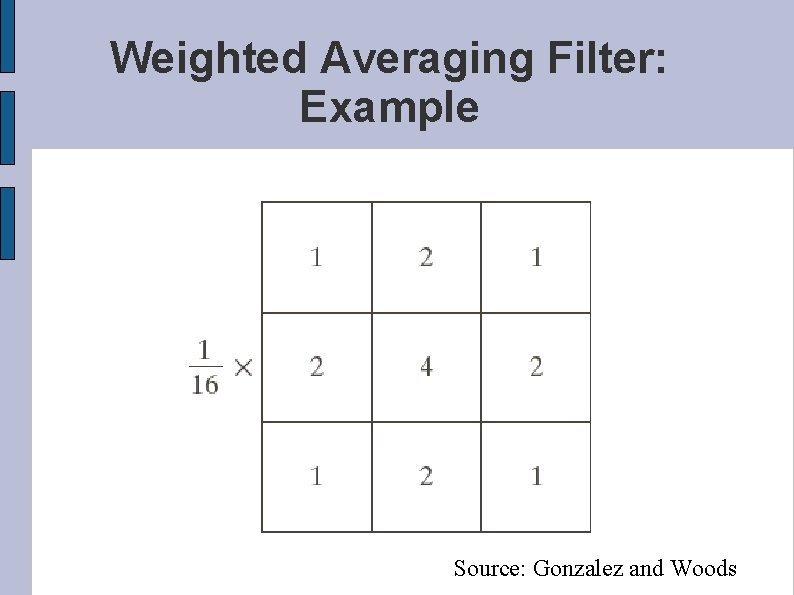
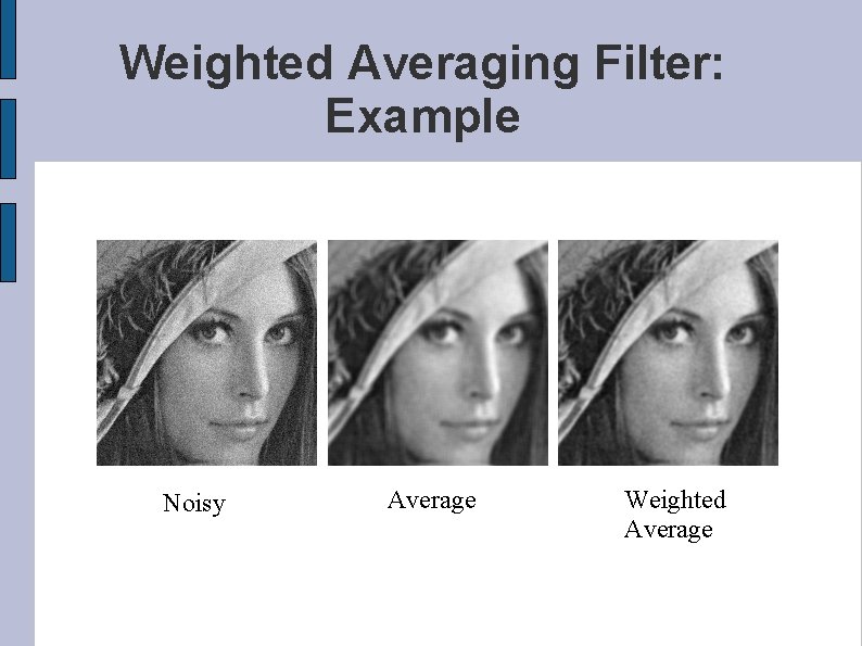
Weighted Average Filter Problem: Simple averaging of neighboring pixels lead to over-smoothing Possible solution: Instead of weighting all neighboring pixels equally, assign higher weights to pixels that are closer to the input pixel

Weighted Averaging Filter: Example Source: Gonzalez and Woods

Weighted Averaging Filter: Example Noisy Average Weighted Average

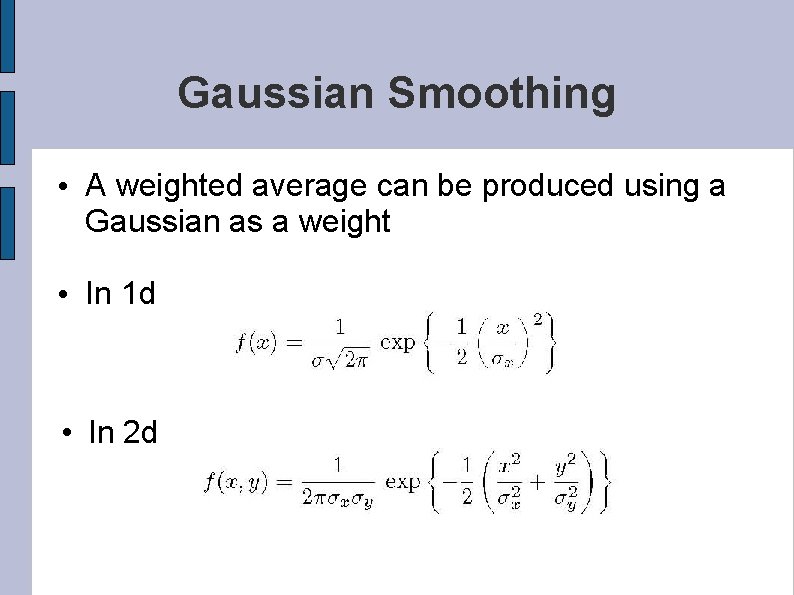
Gaussian Smoothing • A weighted average can be produced using a Gaussian as a weight • In 1 d • In 2 d

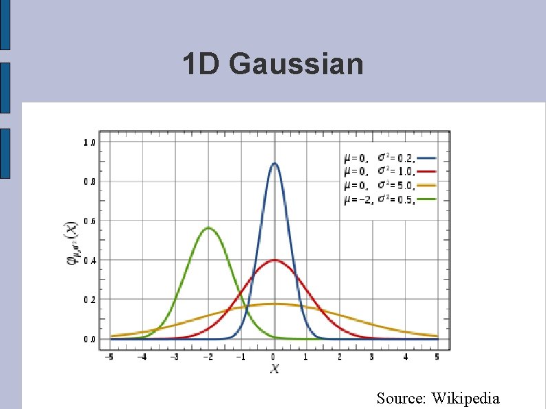
1 D Gaussian Source: Wikipedia

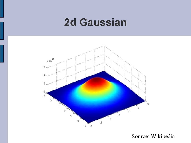
2 d Gaussian Source: Wikipedia

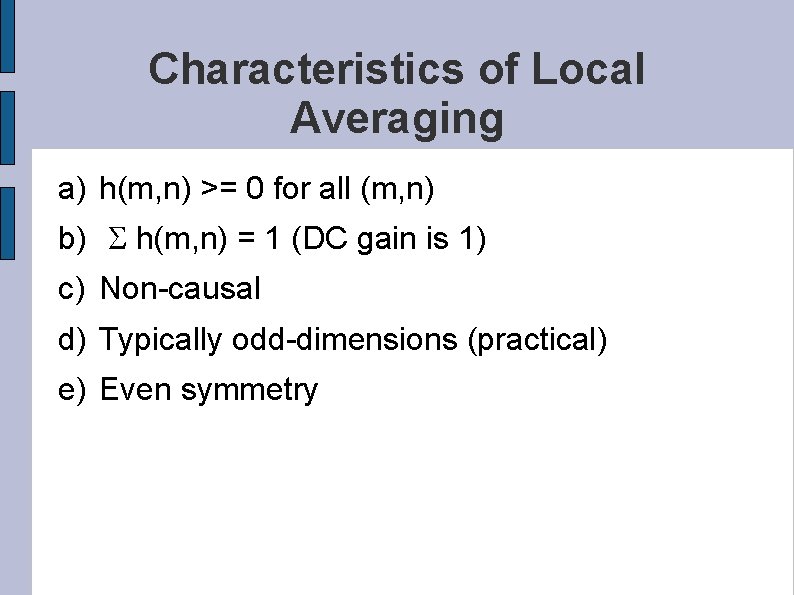
Characteristics of Local Averaging a) h(m, n) >= 0 for all (m, n) b) S h(m, n) = 1 (DC gain is 1) c) Non-causal d) Typically odd-dimensions (practical) e) Even symmetry

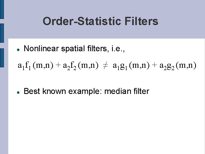
Order-Statistic Filters Nonlinear spatial filters, i. e. , a 1 f 1 (m, n) + a 2 f 2 (m, n) ≠ a 1 g 1 (m, n) + a 2 g 2 (m, n) Best known example: median filter

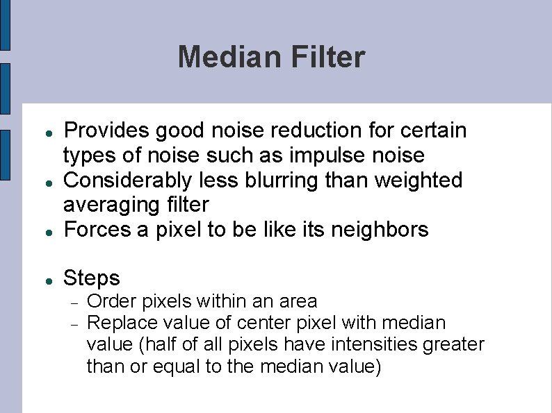
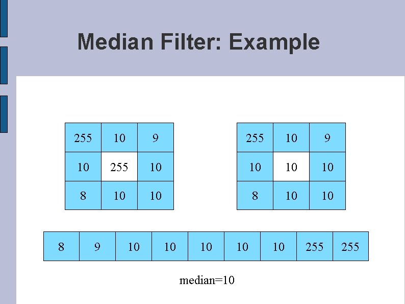
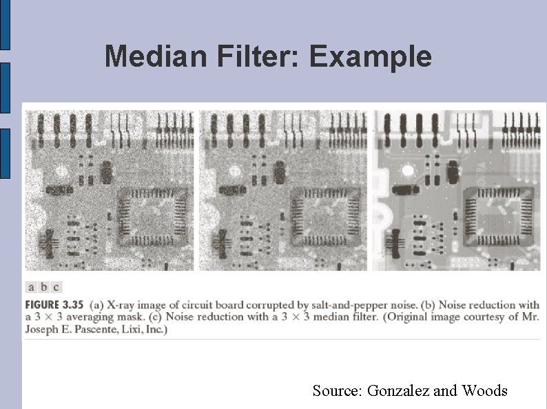
Median Filter Provides good noise reduction for certain types of noise such as impulse noise Considerably less blurring than weighted averaging filter Forces a pixel to be like its neighbors Steps Order pixels within an area Replace value of center pixel with median value (half of all pixels have intensities greater than or equal to the median value)

Median Filter: Example 8 255 10 9 10 255 10 10 8 10 10 9 10 10 10 median=10 10 10 255

Median Filter: Example Source: Gonzalez and Woods

S-statistic Filter • Another method to avoid impact of outliers on smoothing is the S-statistic filter • Basically, only use those values within a region that are within a certain range relative to the mean • Typically, this is done by calculating the m and s of the local region and determining a local average based only on pixels within a certain number of s

Recap: Spatial smoothing filters All of the filters discussed so far are spatial smoothing filters Weight of each pixel in the neighborhood covered by the filter depends on the proximity of the pixel to the center pixel being filtered Typically, the closer the pixel is to the center pixel, the higher the weight

Range Smoothing Filters Problem: oversmoothing of edges and other fine image detail using ideal and Gaussian filters Alternative solution: range smoothing filters Weight of each pixel in the neighborhood covered by the filter depends on the similarity of the pixel's intensity value to that of the center pixel being filtered The closer the pixel's intensity value is to that of the center pixel, the higher the weight

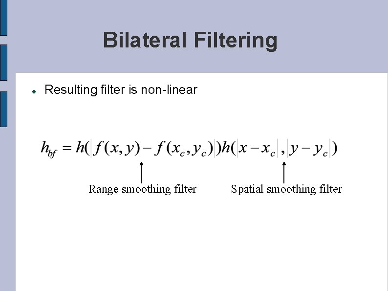
Bilateral Filtering Problem: range smoothing filter simply remaps intensity values No notion of space Poor noise reduction performance (in fact, not really useful by itself) Idea: Combine spatial smoothing filters with range smoothing filters! Good noise reduction (Spatial smoothing) Good edge and detail preservation (Range smoothing)

Bilateral Filtering Resulting filter is non-linear Range smoothing filter Spatial smoothing filter

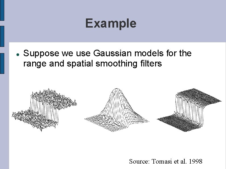
Example Suppose we use Gaussian models for the range and spatial smoothing filters Source: Tomasi et al. 1998

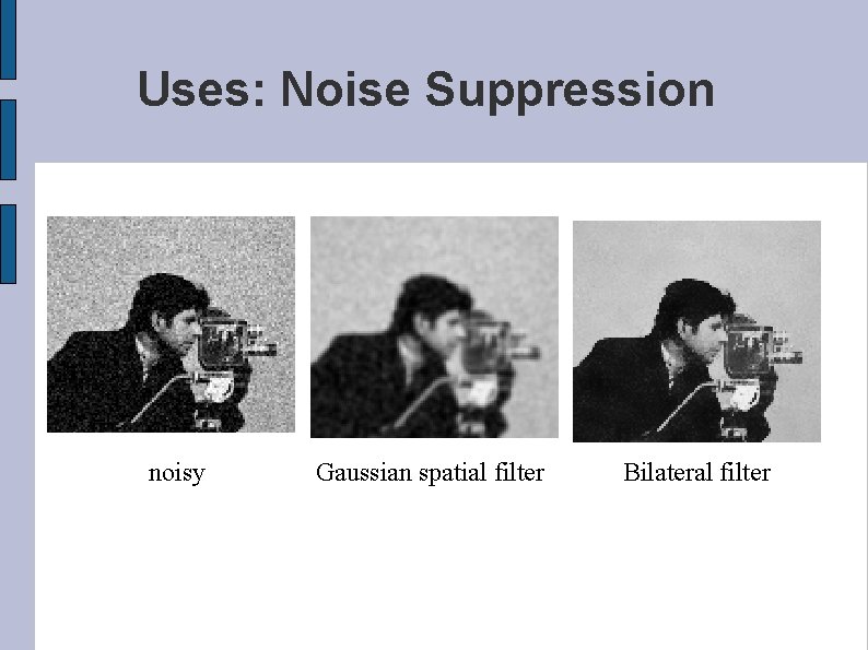
Uses: Noise Suppression noisy Gaussian spatial filter Bilateral filter

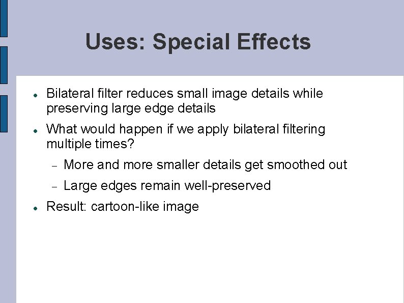
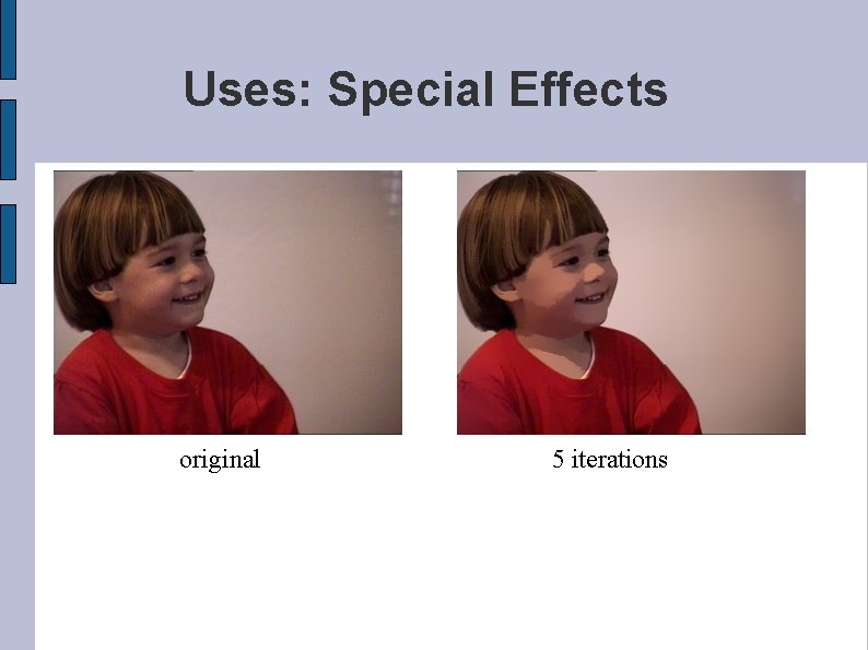
Uses: Special Effects Bilateral filter reduces small image details while preserving large edge details What would happen if we apply bilateral filtering multiple times? More and more smaller details get smoothed out Large edges remain well-preserved Result: cartoon-like image

Uses: Special Effects original 5 iterations

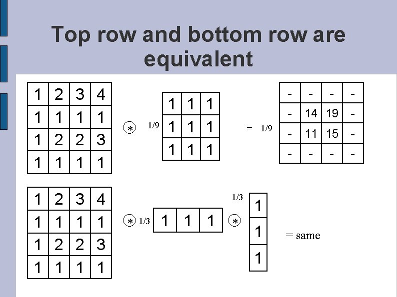
Implementing Symmetrical 2 -D Filters • Large images in use today (e. g. , 1 k x 1 k, 5 k x 5 k, and even larger) require increased computational requirements • Symmetrical filters are commonly used in image processing systems • There is a faster way to implement a 2 -d symmetrical mask using 2 1 -d arrays

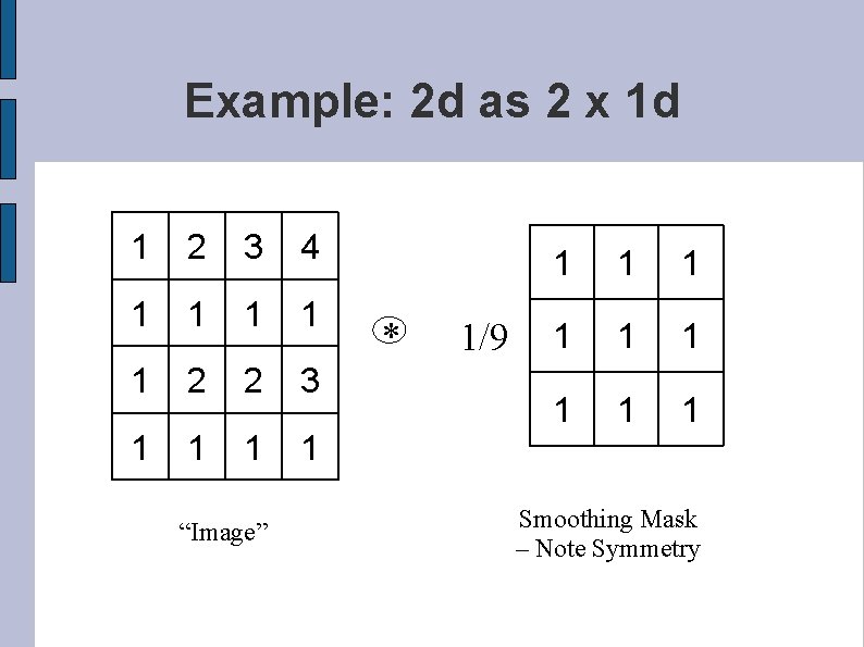
Example: 2 d as 2 x 1 d 1 2 3 4 1 1 1 2 2 3 1 1 “Image” * 1/9 1 1 1 1 1 Smoothing Mask – Note Symmetry

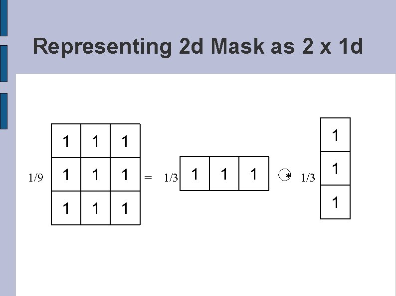
Representing 2 d Mask as 2 x 1 d 1/9 1 1 1 1 1 = 1/3 1 1 1 * 1/3 1 1

Top row and bottom row are equivalent 1 1 1 1 2 1 2 1 3 1 2 1 4 1 3 1 * 1/9 - 1 1 1 1 1 = 1/9 * 1/3 1 1 1 * 1 - 14 19 - - 11 15 - - 1 1 - - 1/3 - = same - -

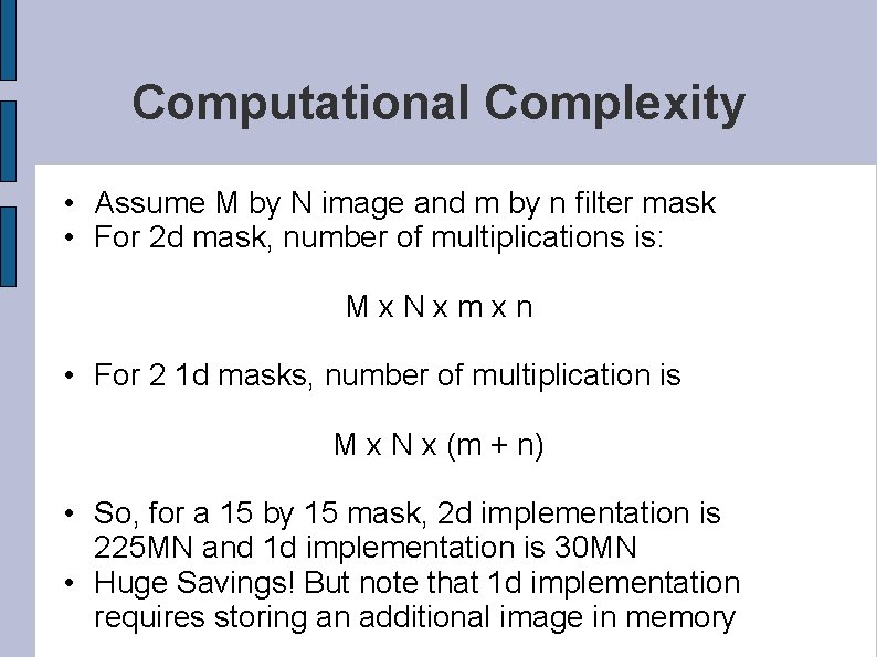
Computational Complexity • Assume M by N image and m by n filter mask • For 2 d mask, number of multiplications is: Mx. Nxmxn • For 2 1 d masks, number of multiplication is M x N x (m + n) • So, for a 15 by 15 mask, 2 d implementation is 225 MN and 1 d implementation is 30 MN • Huge Savings! But note that 1 d implementation requires storing an additional image in memory