Supplement C Special Inventory Models Copyright 2016 Pearson

Supplement C Special Inventory Models Copyright © 2016 Pearson Education, Limited. C-

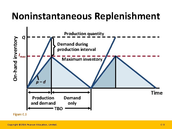
Noninstantaneous Replenishment • Maximum cycle inventory less than Q • Item can be used or sold as it is produced • Production rate, p, exceeds the demand rate, d, so there is a buildup of (p – d) units per time period • Both p and d expressed in same time interval • Buildup continues for Q/p days Copyright © 2016 Pearson Education, Limited. C-2

On-hand inventory Noninstantaneous Replenishment Production quantity Q Demand during production interval Imax Maximum inventory p–d Demand Production only and demand TBO Time Figure C. 1 Copyright © 2016 Pearson Education, Limited. C-3

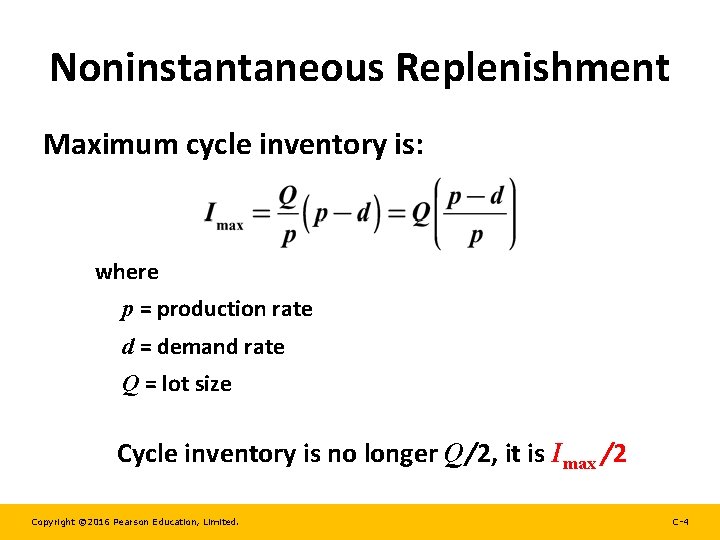
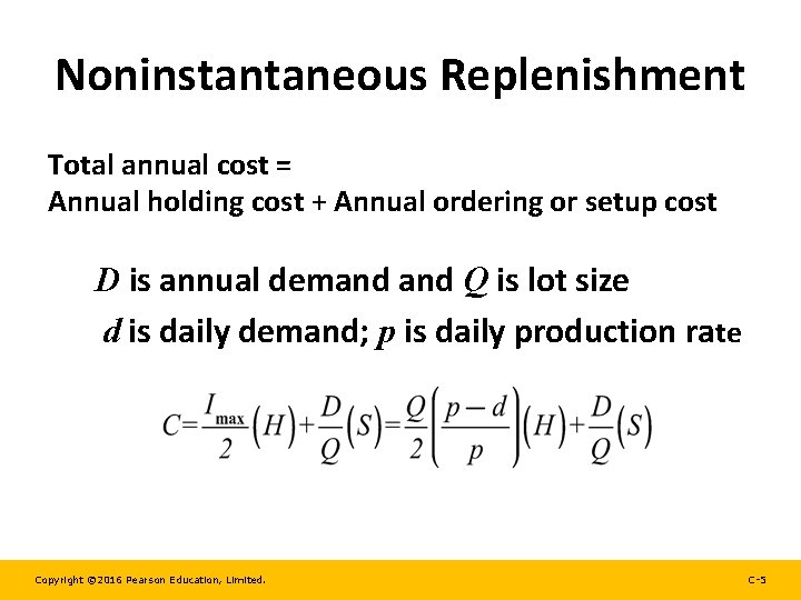
Noninstantaneous Replenishment Maximum cycle inventory is: where p = production rate d = demand rate Q = lot size Cycle inventory is no longer Q/2, it is Imax /2 Copyright © 2016 Pearson Education, Limited. C-4

Noninstantaneous Replenishment Total annual cost = Annual holding cost + Annual ordering or setup cost D is annual demand Q is lot size d is daily demand; p is daily production rate Copyright © 2016 Pearson Education, Limited. C-5

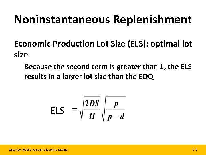
Noninstantaneous Replenishment Economic Production Lot Size (ELS): optimal lot size Because the second term is greater than 1, the ELS results in a larger lot size than the EOQ ELS Copyright © 2016 Pearson Education, Limited. C-6

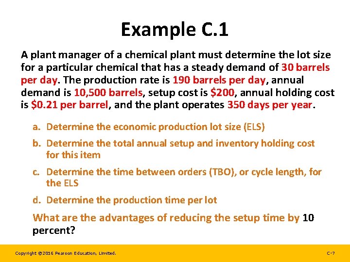
Example C. 1 A plant manager of a chemical plant must determine the lot size for a particular chemical that has a steady demand of 30 barrels per day. The production rate is 190 barrels per day, annual demand is 10, 500 barrels, setup cost is $200, annual holding cost is $0. 21 per barrel, and the plant operates 350 days per year. a. Determine the economic production lot size (ELS) b. Determine the total annual setup and inventory holding cost for this item c. Determine the time between orders (TBO), or cycle length, for the ELS d. Determine the production time per lot What are the advantages of reducing the setup time by 10 percent? Copyright © 2016 Pearson Education, Limited. C-7

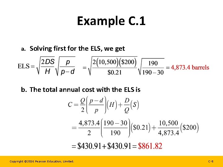
Example C. 1 a. Solving first for the ELS, we get b. The total annual cost with the ELS is Copyright © 2016 Pearson Education, Limited. C-8

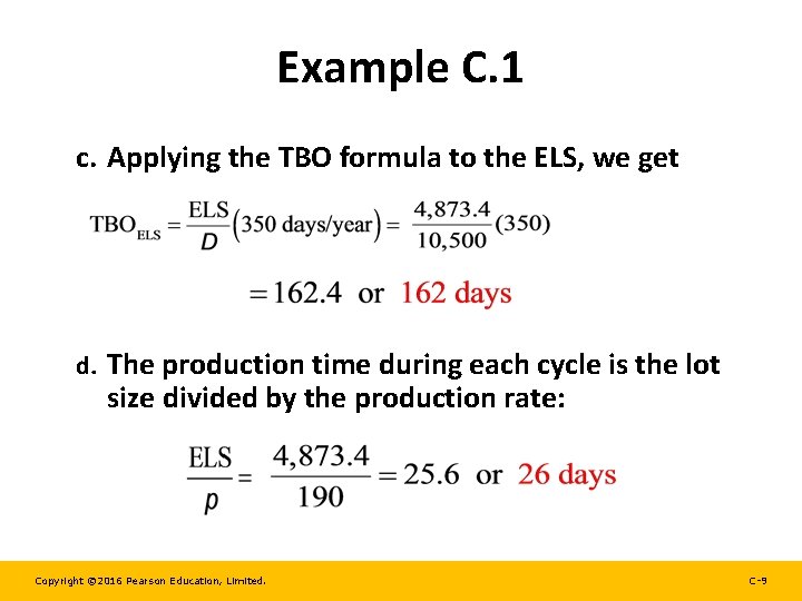
Example C. 1 c. Applying the TBO formula to the ELS, we get d. The production time during each cycle is the lot size divided by the production rate: Copyright © 2016 Pearson Education, Limited. C-9

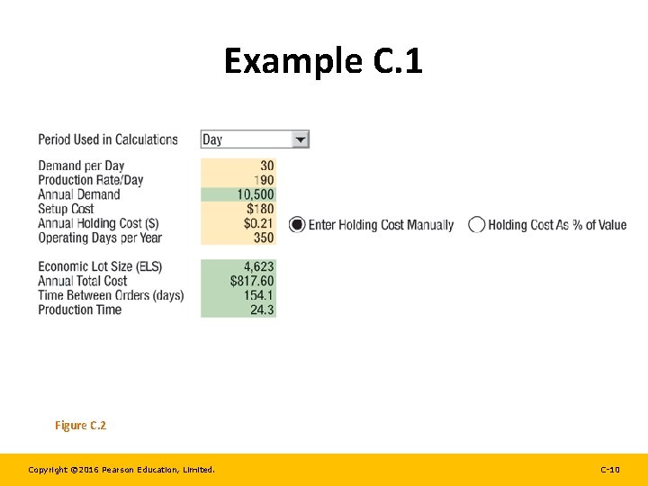
Example C. 1 Figure C. 2 Copyright © 2016 Pearson Education, Limited. C-10

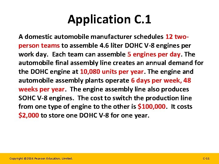
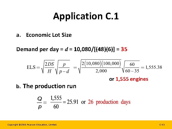
Application C. 1 A domestic automobile manufacturer schedules 12 twoperson teams to assemble 4. 6 liter DOHC V-8 engines per work day. Each team can assemble 5 engines per day. The automobile final assembly line creates an annual demand for the DOHC engine at 10, 080 units per year. The engine and automobile assembly plants operate 6 days per week, 48 weeks per year. The engine assembly line also produces SOHC V-8 engines. The cost to switch the production line from one type of engine to the other is $100, 000. It costs $2, 000 to store one DOHC V-8 for one year. Copyright © 2016 Pearson Education, Limited. C-11

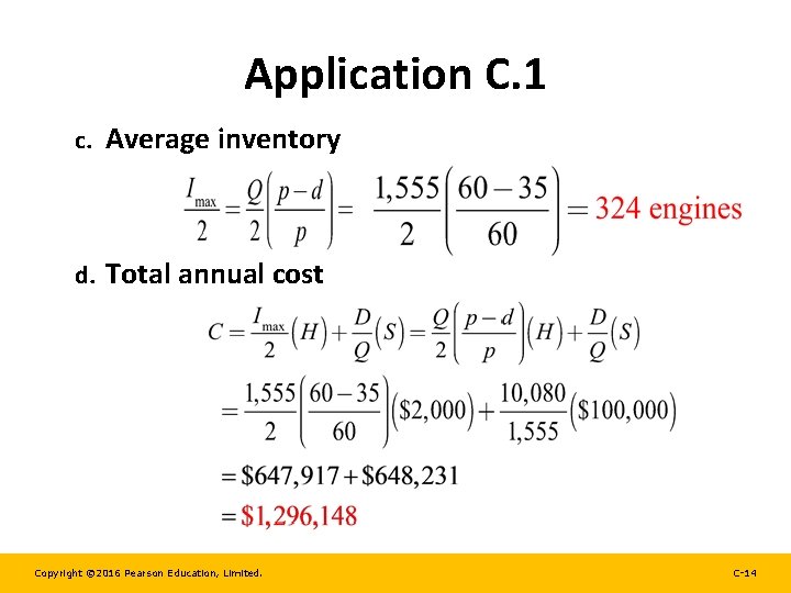
Application C. 1 a. What is the economic lot size? b. How long is the production run? c. What is the average quantity in inventory? d. What is the total annual cost? Copyright © 2016 Pearson Education, Limited. C-12

Application C. 1 a. Economic Lot Size Demand per day = d = 10, 080/[(48)(6)] = 35 b. The production run Copyright © 2016 Pearson Education, Limited. or 1, 555 engines C-13

Application C. 1 c. Average inventory d. Total annual cost Copyright © 2016 Pearson Education, Limited. C-14

Quantity Discounts • Price incentives to purchase large quantities create pressure to maintain a large inventory • Item’s price is no longer fixed – If the order quantity is increased enough, then the price per unit is discounted – A new approach is needed to find the best lot size that balances: • Advantages of lower prices for purchased materials and fewer orders • Disadvantages of the increased cost of holding more inventory Copyright © 2016 Pearson Education, Limited. C-15

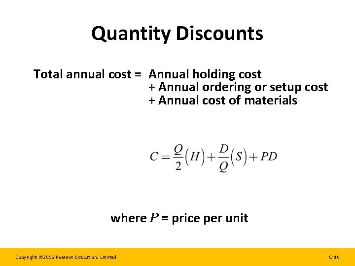
Quantity Discounts Total annual cost = Annual holding cost + Annual ordering or setup cost + Annual cost of materials where P = price per unit Copyright © 2016 Pearson Education, Limited. C-16

Quantity Discounts • Unit holding cost (H) is usually expressed as a percentage of unit price • The lower the unit price (P) is, the lower the unit holding cost (H) is Copyright © 2016 Pearson Education, Limited. C-17

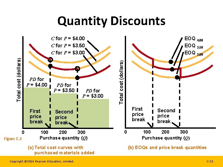
Quantity Discounts • The total cost equation yields U-shape total cost curves – There are cost curves for each price level – The feasible total cost begins with the top curve, then drops down, curve by curve, at the price breaks – EOQs do not necessarily produce the best lot size • The EOQ at a particular price level may not be feasible • The EOQ at a particular price level may be feasible but may not be the best lot size Copyright © 2016 Pearson Education, Limited. C-18

Quantity Discounts Two-Step Solution Procedure Step 1. Beginning with lowest price, calculate the EOQ for each price level until a feasible EOQ is found. It is feasible if it lies in the range corresponding to its price. Each subsequent EOQ is smaller than the previous one, because P, and thus H, gets larger and because the larger H is in the denominator of the EOQ formula. Copyright © 2016 Pearson Education, Limited. C-19

Quantity Discounts Step 2. If the first feasible EOQ found is for the lowest price level, this quantity is the best lot size. Otherwise, calculate the total cost for the first feasible EOQ and for the larger price break quantity at each lower price level. The quantity with the lowest total cost is optimal. Copyright © 2016 Pearson Education, Limited. C-20

Quantity Discounts EOQ 4. 00 EOQ 3. 50 EOQ 3. 00 PD for P = $4. 00 First price break 0 Figure C. 3 PD for P = $3. 50 PD for P = $3. 00 Total cost (dollars) C for P = $4. 00 C for P = $3. 50 C for P = $3. 00 First price break Second price break 100 200 300 Purchase quantity (Q) (a) Total cost curves with purchased materials added Copyright © 2016 Pearson Education, Limited. 0 Second price break 100 200 300 Purchase quantity (Q) (b) EOQs and price break quantities C-21

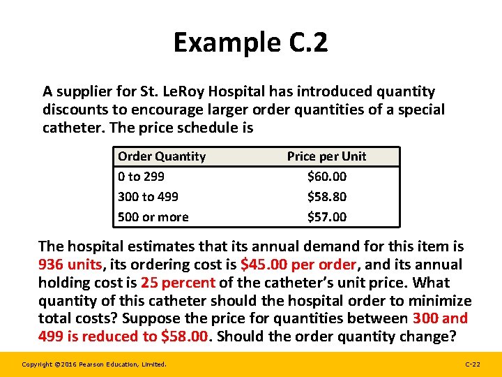
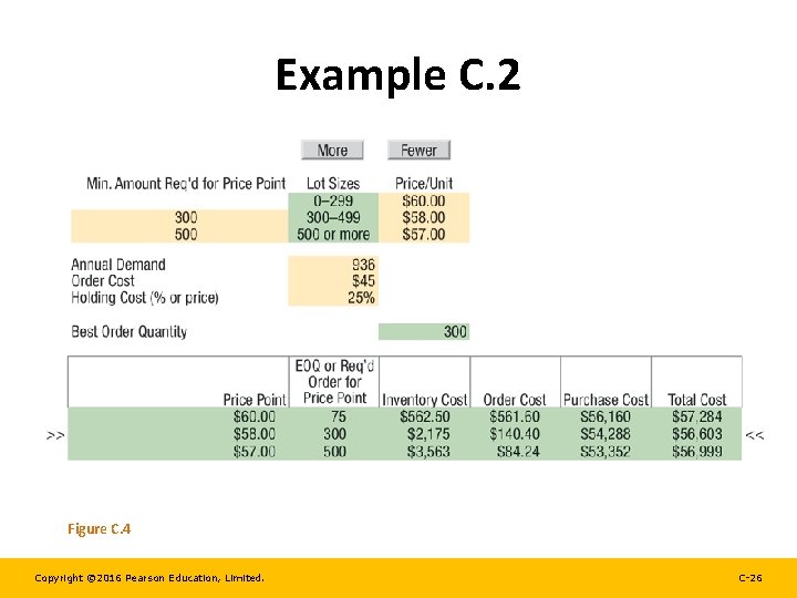
Example C. 2 A supplier for St. Le. Roy Hospital has introduced quantity discounts to encourage larger order quantities of a special catheter. The price schedule is Order Quantity 0 to 299 300 to 499 500 or more Price per Unit $60. 00 $58. 80 $57. 00 The hospital estimates that its annual demand for this item is 936 units, its ordering cost is $45. 00 per order, and its annual holding cost is 25 percent of the catheter’s unit price. What quantity of this catheter should the hospital order to minimize total costs? Suppose the price for quantities between 300 and 499 is reduced to $58. 00. Should the order quantity change? Copyright © 2016 Pearson Education, Limited. C-22

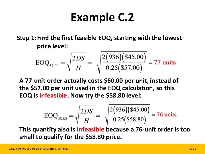
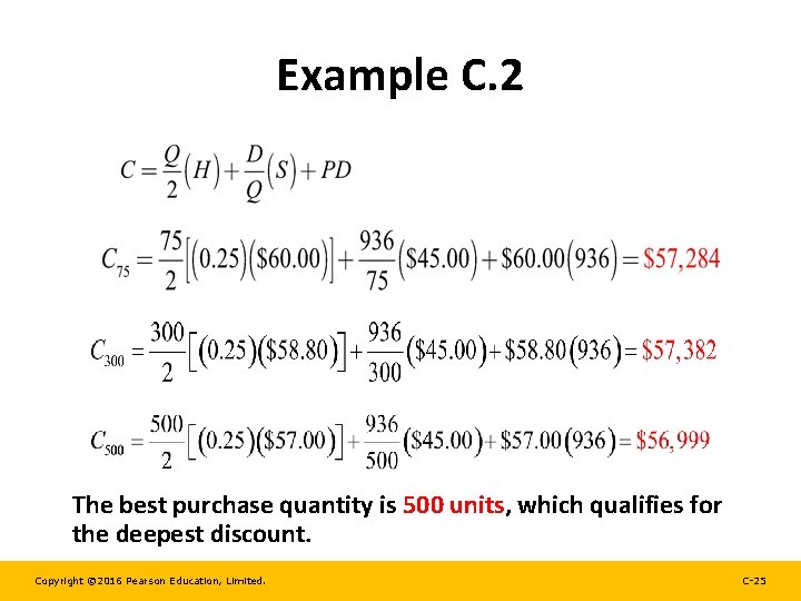
Example C. 2 Step 1: Find the first feasible EOQ, starting with the lowest price level: A 77 -unit order actually costs $60. 00 per unit, instead of the $57. 00 per unit used in the EOQ calculation, so this EOQ is infeasible. Now try the $58. 80 level: This quantity also is infeasible because a 76 -unit order is too small to qualify for the $58. 80 price. Copyright © 2016 Pearson Education, Limited. C-23

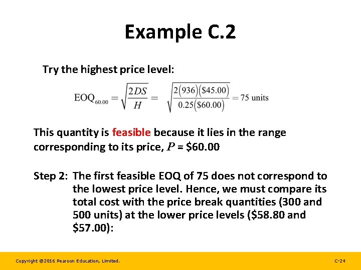
Example C. 2 Try the highest price level: This quantity is feasible because it lies in the range corresponding to its price, P = $60. 00 Step 2: The first feasible EOQ of 75 does not correspond to the lowest price level. Hence, we must compare its total cost with the price break quantities (300 and 500 units) at the lower price levels ($58. 80 and $57. 00): Copyright © 2016 Pearson Education, Limited. C-24

Example C. 2 The best purchase quantity is 500 units, which qualifies for the deepest discount. Copyright © 2016 Pearson Education, Limited. C-25

Example C. 2 Figure C. 4 Copyright © 2016 Pearson Education, Limited. C-26

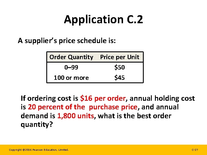
Application C. 2 A supplier’s price schedule is: Order Quantity 0– 99 100 or more Price per Unit $50 $45 If ordering cost is $16 per order, annual holding cost is 20 percent of the purchase price, and annual demand is 1, 800 units, what is the best order quantity? Copyright © 2016 Pearson Education, Limited. C-27

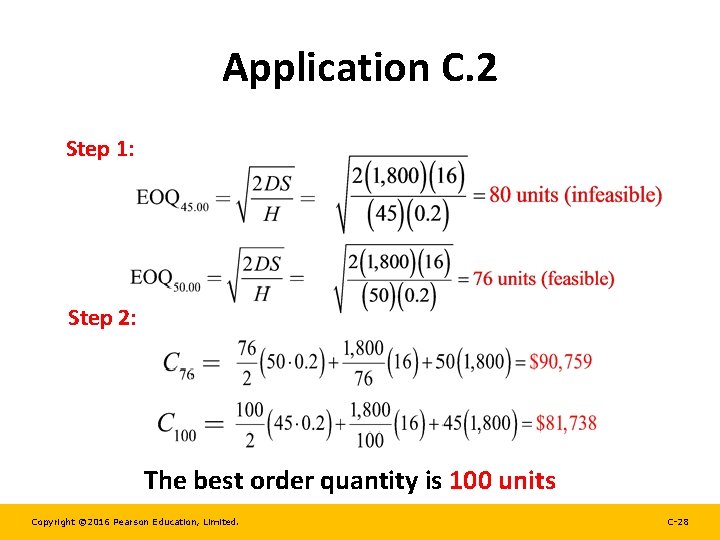
Application C. 2 Step 1: Step 2: The best order quantity is 100 units Copyright © 2016 Pearson Education, Limited. C-28

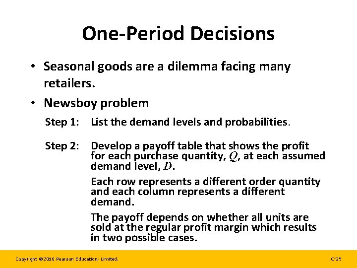
One-Period Decisions • Seasonal goods are a dilemma facing many retailers. • Newsboy problem Step 1: List the demand levels and probabilities. Step 2: Develop a payoff table that shows the profit for each purchase quantity, Q, at each assumed demand level, D. Each row represents a different order quantity and each column represents a different demand. The payoff depends on whether all units are sold at the regular profit margin which results in two possible cases. Copyright © 2016 Pearson Education, Limited. C-29

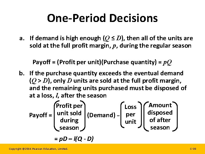
One-Period Decisions a. If demand is high enough (Q ≤ D), then all of the units are sold at the full profit margin, p, during the regular season Payoff = (Profit per unit)(Purchase quantity) = p. Q b. If the purchase quantity exceeds the eventual demand (Q > D), only D units are sold at the full profit margin, and the remaining units purchased must be disposed of at a loss, l, after the season Amount Profit per Loss disposed Payoff = unit sold (Demand) – per of after during unit season = p. D – l(Q - D) Copyright © 2016 Pearson Education, Limited. C-30

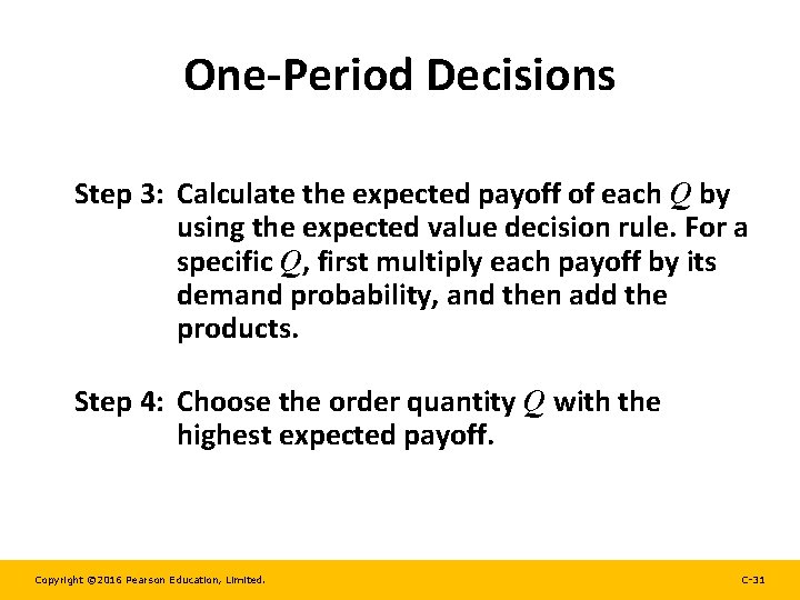
One-Period Decisions Step 3: Calculate the expected payoff of each Q by using the expected value decision rule. For a specific Q, first multiply each payoff by its demand probability, and then add the products. Step 4: Choose the order quantity Q with the highest expected payoff. Copyright © 2016 Pearson Education, Limited. C-31

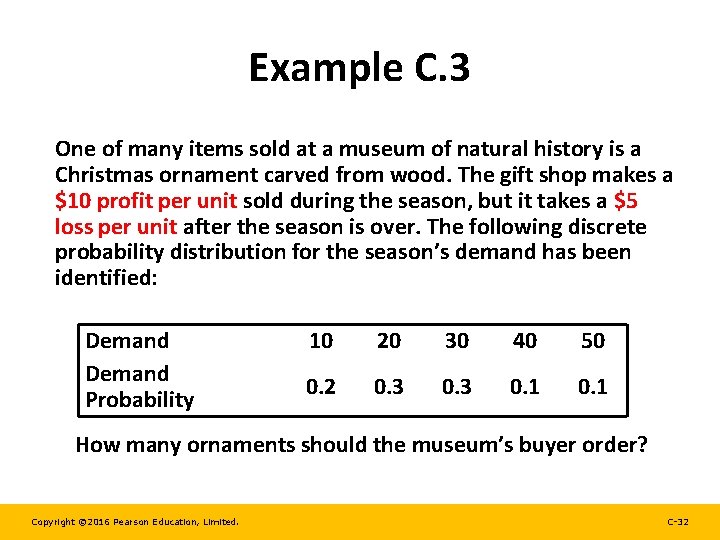
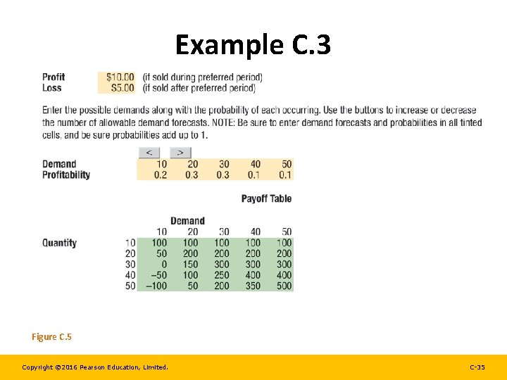
Example C. 3 One of many items sold at a museum of natural history is a Christmas ornament carved from wood. The gift shop makes a $10 profit per unit sold during the season, but it takes a $5 loss per unit after the season is over. The following discrete probability distribution for the season’s demand has been identified: Demand Probability 10 20 30 40 50 0. 2 0. 3 0. 1 How many ornaments should the museum’s buyer order? Copyright © 2016 Pearson Education, Limited. C-32

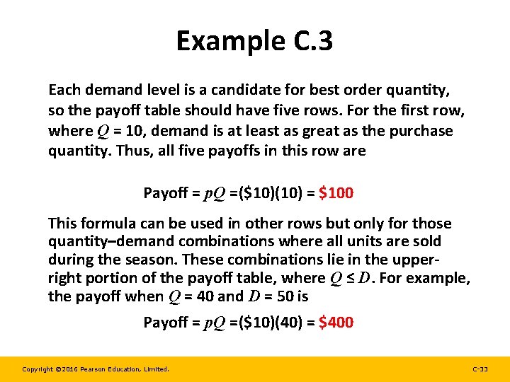
Example C. 3 Each demand level is a candidate for best order quantity, so the payoff table should have five rows. For the first row, where Q = 10, demand is at least as great as the purchase quantity. Thus, all five payoffs in this row are Payoff = p. Q =($10)(10) = $100 This formula can be used in other rows but only for those quantity–demand combinations where all units are sold during the season. These combinations lie in the upperright portion of the payoff table, where Q ≤ D. For example, the payoff when Q = 40 and D = 50 is Payoff = p. Q =($10)(40) = $400 Copyright © 2016 Pearson Education, Limited. C-33

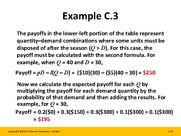
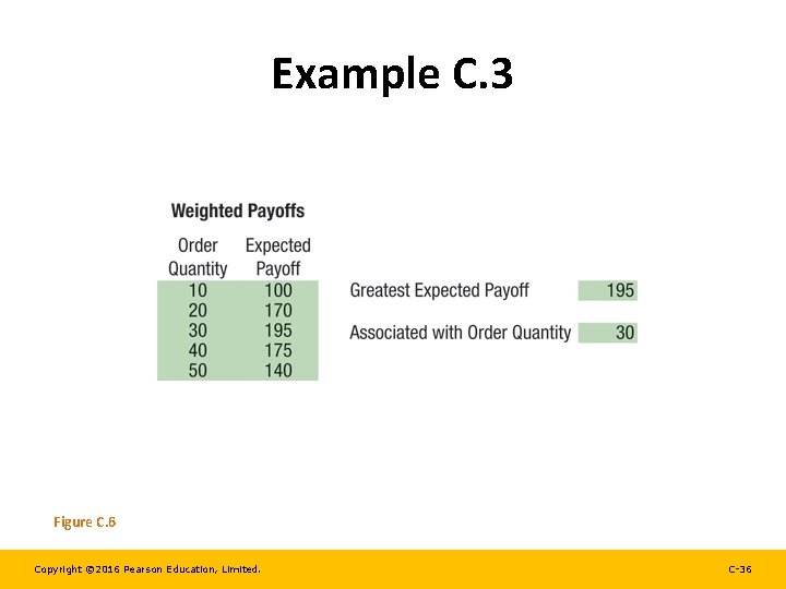
Example C. 3 The payoffs in the lower-left portion of the table represent quantity–demand combinations where some units must be disposed of after the season (Q > D). For this case, the payoff must be calculated with the second formula. For example, when Q = 40 and D = 30, Payoff = p. D – l(Q – D) = ($10)(30) – ($5)(40 – 30) = $250 Now we calculate the expected payoff for each Q by multiplying the payoff for each demand quantity by the probability of that demand then adding the results. For example, for Q = 30, Payoff = 0. 2($0) + 0. 3($150) + 0. 3($300) + 0. 1($300) = $195 Copyright © 2016 Pearson Education, Limited. C-34

Example C. 3 Figure C. 5 Copyright © 2016 Pearson Education, Limited. C-35

Example C. 3 Figure C. 6 Copyright © 2016 Pearson Education, Limited. C-36

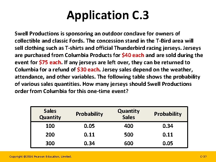
Application C. 3 Swell Productions is sponsoring an outdoor conclave for owners of collectible and classic Fords. The concession stand in the T-Bird area will sell clothing such as T-shirts and official Thunderbird racing jerseys. Jerseys are purchased from Columbia Products for $40 each and are sold during the event for $75 each. If any jerseys are left over, they can be returned to Columbia for a refund of $30 each. Jersey sales depend on the weather, attendance, and other variables. The following table shows the probability of various sales quantities. How many jerseys should Swell Productions order from Columbia for this one-time event? Sales Quantity 100 200 300 Copyright © 2016 Pearson Education, Limited. Probability 0. 05 0. 11 0. 34 Quantity Sales 400 500 600 Probability 0. 34 0. 11 0. 05 C-37

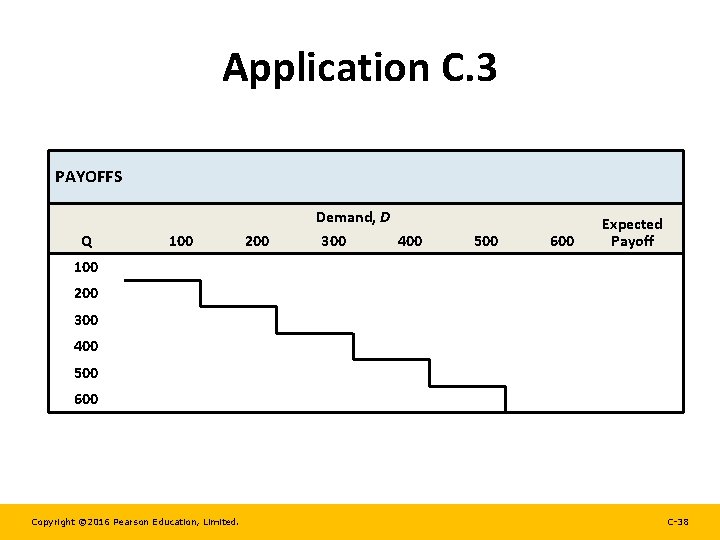
Application C. 3 PAYOFFS Demand, D Q 100 200 300 400 500 600 Expected Payoff 100 200 300 400 500 600 Copyright © 2016 Pearson Education, Limited. C-38

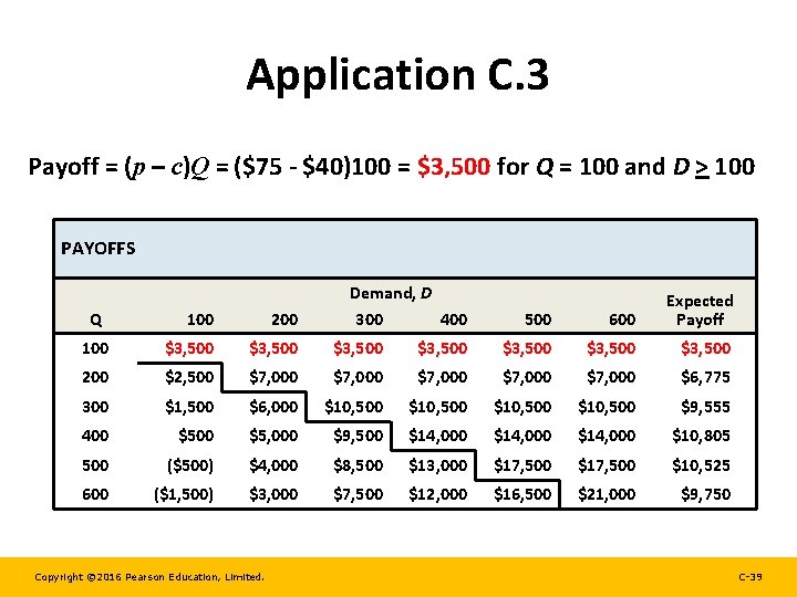
Application C. 3 Payoff = (p – c)Q = ($75 - $40)100 = $3, 500 for Q = 100 and D > 100 PAYOFFS Demand, D 100 200 300 400 500 600 Expected Payoff 100 $3, 500 $3, 500 200 $2, 500 $7, 000 $7, 000 $6, 775 300 $1, 500 $6, 000 $10, 500 $9, 555 400 $5, 000 $9, 500 $14, 000 $10, 805 500 ($500) $4, 000 $8, 500 $13, 000 $17, 500 $10, 525 600 ($1, 500) $3, 000 $7, 500 $12, 000 $16, 500 $21, 000 $9, 750 Q Copyright © 2016 Pearson Education, Limited. C-39

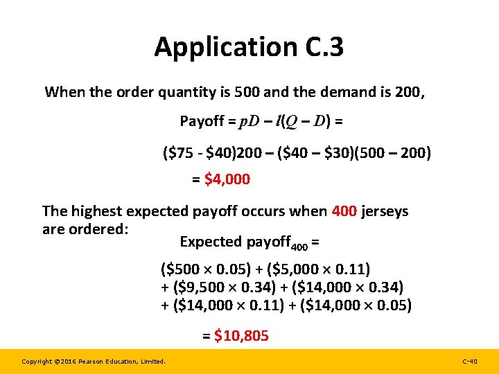
Application C. 3 When the order quantity is 500 and the demand is 200, Payoff = p. D – l(Q – D) = ($75 - $40)200 – ($40 – $30)(500 – 200) = $4, 000 The highest expected payoff occurs when 400 jerseys are ordered: Expected payoff 400 = ($500 0. 05) + ($5, 000 0. 11) + ($9, 500 0. 34) + ($14, 000 0. 11) + ($14, 000 0. 05) = $10, 805 Copyright © 2016 Pearson Education, Limited. C-40

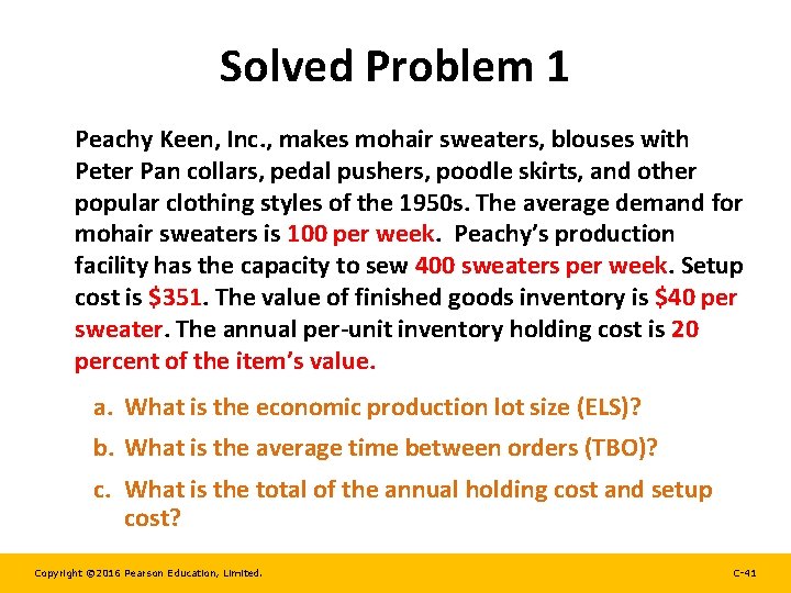
Solved Problem 1 Peachy Keen, Inc. , makes mohair sweaters, blouses with Peter Pan collars, pedal pushers, poodle skirts, and other popular clothing styles of the 1950 s. The average demand for mohair sweaters is 100 per week. Peachy’s production facility has the capacity to sew 400 sweaters per week. Setup cost is $351. The value of finished goods inventory is $40 per sweater. The annual per-unit inventory holding cost is 20 percent of the item’s value. a. What is the economic production lot size (ELS)? b. What is the average time between orders (TBO)? c. What is the total of the annual holding cost and setup cost? Copyright © 2016 Pearson Education, Limited. C-41

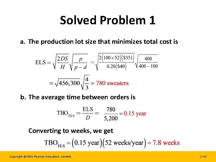
Solved Problem 1 a. The production lot size that minimizes total cost is b. The average time between orders is Converting to weeks, we get Copyright © 2016 Pearson Education, Limited. C-42

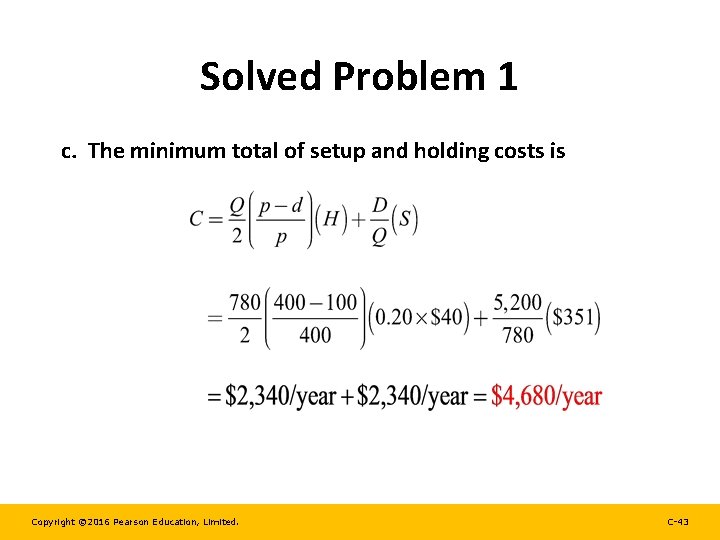
Solved Problem 1 c. The minimum total of setup and holding costs is Copyright © 2016 Pearson Education, Limited. C-43

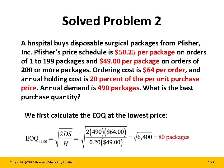
Solved Problem 2 A hospital buys disposable surgical packages from Pfisher, Inc. Pfisher’s price schedule is $50. 25 per package on orders of 1 to 199 packages and $49. 00 per package on orders of 200 or more packages. Ordering cost is $64 per order, and annual holding cost is 20 percent of the per unit purchase price. Annual demand is 490 packages. What is the best purchase quantity? We first calculate the EOQ at the lowest price: Copyright © 2016 Pearson Education, Limited. C-44

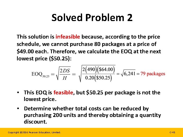
Solved Problem 2 This solution is infeasible because, according to the price schedule, we cannot purchase 80 packages at a price of $49. 00 each. Therefore, we calculate the EOQ at the next lowest price ($50. 25): • This EOQ is feasible, but $50. 25 per package is not the lowest price. • Determine whether total costs can be reduced by purchasing 200 units and thereby obtaining a quantity discount. Copyright © 2016 Pearson Education, Limited. C-45

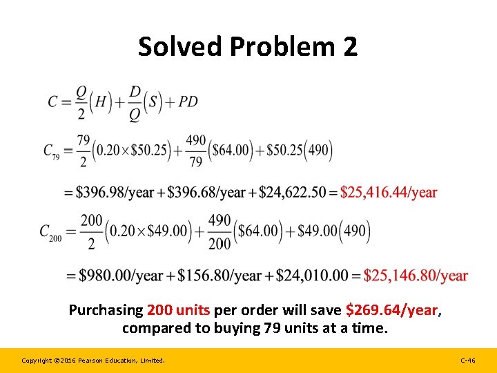
Solved Problem 2 Purchasing 200 units per order will save $269. 64/year, compared to buying 79 units at a time. Copyright © 2016 Pearson Education, Limited. C-46