Special Inventory Models Supplement E To Accompany Krajewski

On-hand inventory Special Inventory Models Production quantity Q Demand during production interval p–d Time

On-hand inventory Special Inventory Models Production quantity Q Demand during production interval Imax Maximum

Special Inventory Models Economic Production Lot Size Demand = 30 barrels/day Production rate =

Special Inventory Models Quantity Discounts Figure E. 3 EOQ 4. 00 EOQ 3. 50

Special Inventory Models Quantity Discounts Order Quantity Price per Unit 0 – 299 300

Special Inventory Models Quantity Discounts Order Quantity 0 – 299 300 – 499 500

Special Inventory Models One-Period Decisions Demand 10 20 30 40 50 Demand Probability 0.

Slides: 32

Download presentation

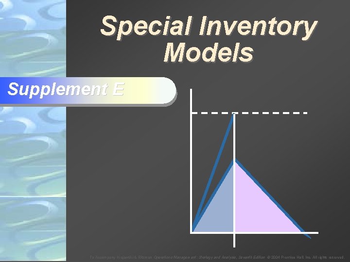
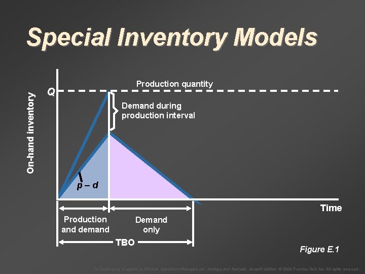
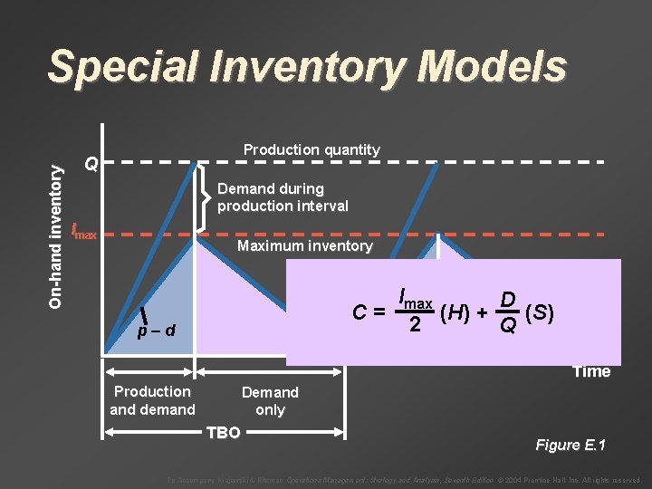
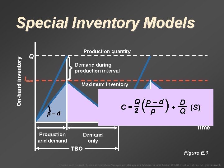
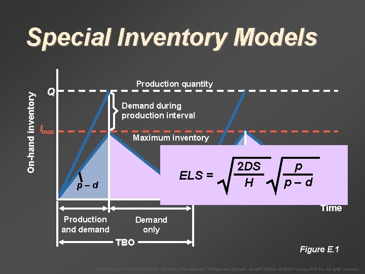
On-hand inventory Special Inventory Models Production quantity Q Demand during production interval p–d Time Production and demand Demand only TBO Figure E. 1 To Accompany Krajewski & Ritzman Operations Management: Strategy and Analysis, Seventh Edition © 2004 Prentice Hall, Inc. All rights reserved.

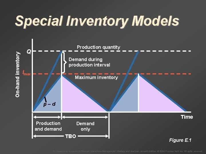
On-hand inventory Special Inventory Models Production quantity Q Demand during production interval Imax Maximum inventory p–d Time Production and demand Demand only TBO Figure E. 1 To Accompany Krajewski & Ritzman Operations Management: Strategy and Analysis, Seventh Edition © 2004 Prentice Hall, Inc. All rights reserved.

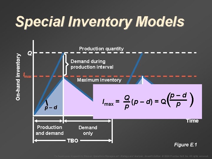
On-hand inventory Special Inventory Models Production quantity Q Demand during production interval Imax Maximum inventory ( p–d Q Imax = (p – d) = Q p p p–d ) Time Production and demand Demand only TBO Figure E. 1 To Accompany Krajewski & Ritzman Operations Management: Strategy and Analysis, Seventh Edition © 2004 Prentice Hall, Inc. All rights reserved.

On-hand inventory Special Inventory Models Production quantity Q Demand during production interval Imax Maximum inventory Imax D C= (H) + (S) 2 Q p–d Time Production and demand Demand only TBO Figure E. 1 To Accompany Krajewski & Ritzman Operations Management: Strategy and Analysis, Seventh Edition © 2004 Prentice Hall, Inc. All rights reserved.

On-hand inventory Special Inventory Models Production quantity Q Demand during production interval Imax Maximum inventory ( Q p–d C =2 p p–d ) D + (S) Q Time Production and demand Demand only TBO Figure E. 1 To Accompany Krajewski & Ritzman Operations Management: Strategy and Analysis, Seventh Edition © 2004 Prentice Hall, Inc. All rights reserved.

On-hand inventory Special Inventory Models Production quantity Q Demand during production interval Imax Maximum inventory ELS = p–d 2 DS H p p–d Time Production and demand Demand only TBO Figure E. 1 To Accompany Krajewski & Ritzman Operations Management: Strategy and Analysis, Seventh Edition © 2004 Prentice Hall, Inc. All rights reserved.

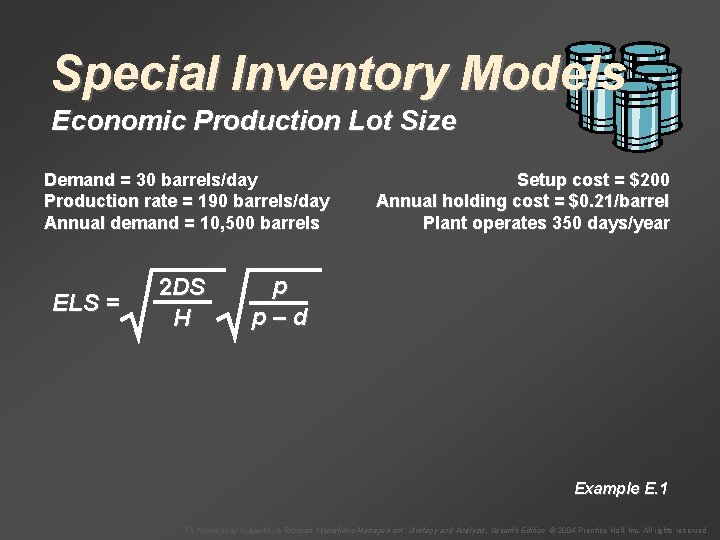
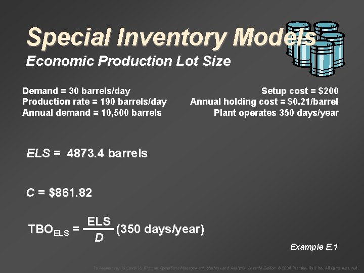
Special Inventory Models Economic Production Lot Size Demand = 30 barrels/day Production rate = 190 barrels/day Annual demand = 10, 500 barrels ELS = 2 DS H Setup cost = $200 Annual holding cost = $0. 21/barrel Plant operates 350 days/year p p–d Example E. 1 To Accompany Krajewski & Ritzman Operations Management: Strategy and Analysis, Seventh Edition © 2004 Prentice Hall, Inc. All rights reserved.

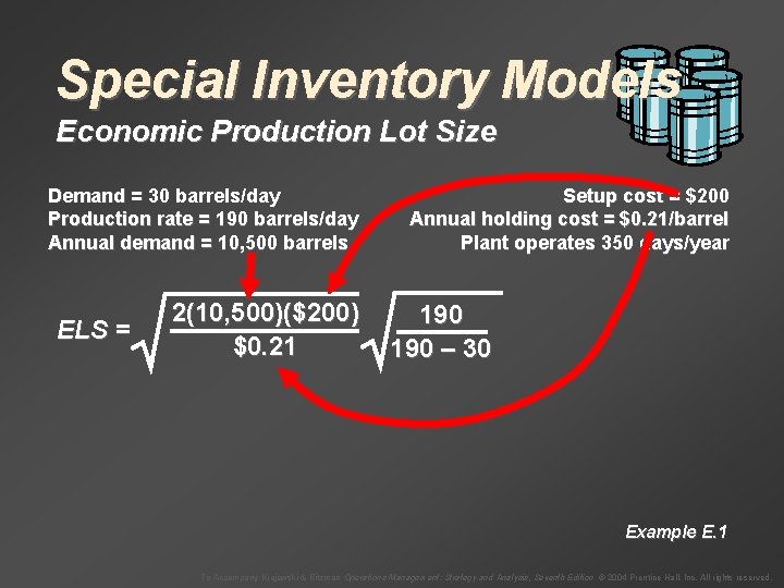
Special Inventory Models Economic Production Lot Size Demand = 30 barrels/day Production rate = 190 barrels/day Annual demand = 10, 500 barrels ELS = 2(10, 500)($200) $0. 21 Setup cost = $200 Annual holding cost = $0. 21/barrel Plant operates 350 days/year 190 – 30 Example E. 1 To Accompany Krajewski & Ritzman Operations Management: Strategy and Analysis, Seventh Edition © 2004 Prentice Hall, Inc. All rights reserved.

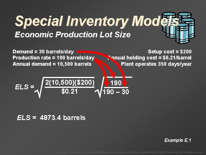
Special Inventory Models Economic Production Lot Size Demand = 30 barrels/day Production rate = 190 barrels/day Annual demand = 10, 500 barrels ELS = 2(10, 500)($200) $0. 21 Setup cost = $200 Annual holding cost = $0. 21/barrel Plant operates 350 days/year 190 – 30 ELS = 4873. 4 barrels Example E. 1 To Accompany Krajewski & Ritzman Operations Management: Strategy and Analysis, Seventh Edition © 2004 Prentice Hall, Inc. All rights reserved.

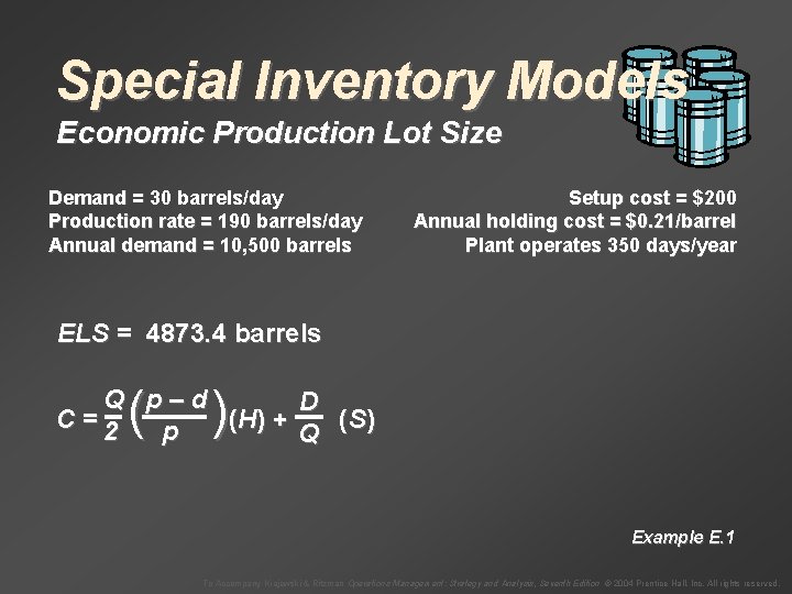
Special Inventory Models Economic Production Lot Size Demand = 30 barrels/day Production rate = 190 barrels/day Annual demand = 10, 500 barrels Setup cost = $200 Annual holding cost = $0. 21/barrel Plant operates 350 days/year ELS = 4873. 4 barrels ( ) Q p–d D C =2 (H ) + ( S) p Q Example E. 1 To Accompany Krajewski & Ritzman Operations Management: Strategy and Analysis, Seventh Edition © 2004 Prentice Hall, Inc. All rights reserved.

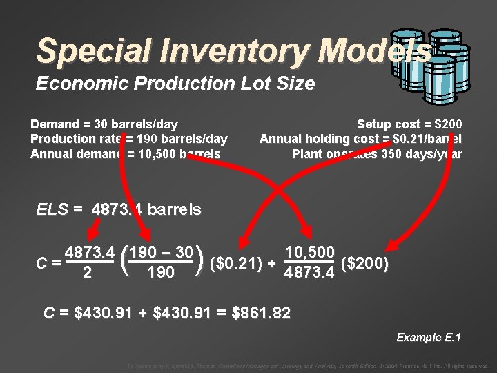
Special Inventory Models Economic Production Lot Size Demand = 30 barrels/day Production rate = 190 barrels/day Annual demand = 10, 500 barrels Setup cost = $200 Annual holding cost = $0. 21/barrel Plant operates 350 days/year ELS = 4873. 4 barrels ( ) 10, 500 4873. 4 190 – 30 C= ($0. 21) + ($200) 4873. 4 2 190 C = $430. 91 + $430. 91 = $861. 82 Example E. 1 To Accompany Krajewski & Ritzman Operations Management: Strategy and Analysis, Seventh Edition © 2004 Prentice Hall, Inc. All rights reserved.

Special Inventory Models Economic Production Lot Size Demand = 30 barrels/day Production rate = 190 barrels/day Annual demand = 10, 500 barrels Setup cost = $200 Annual holding cost = $0. 21/barrel Plant operates 350 days/year ELS = 4873. 4 barrels C = $861. 82 ELS TBOELS = (350 days/year) D Example E. 1 To Accompany Krajewski & Ritzman Operations Management: Strategy and Analysis, Seventh Edition © 2004 Prentice Hall, Inc. All rights reserved.

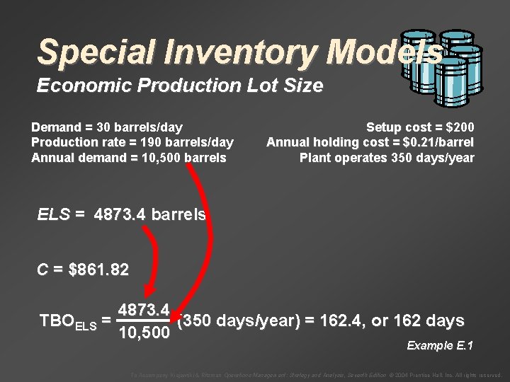
Special Inventory Models Economic Production Lot Size Demand = 30 barrels/day Production rate = 190 barrels/day Annual demand = 10, 500 barrels Setup cost = $200 Annual holding cost = $0. 21/barrel Plant operates 350 days/year ELS = 4873. 4 barrels C = $861. 82 4873. 4 TBOELS = (350 days/year) = 162. 4, or 162 days 10, 500 Example E. 1 To Accompany Krajewski & Ritzman Operations Management: Strategy and Analysis, Seventh Edition © 2004 Prentice Hall, Inc. All rights reserved.

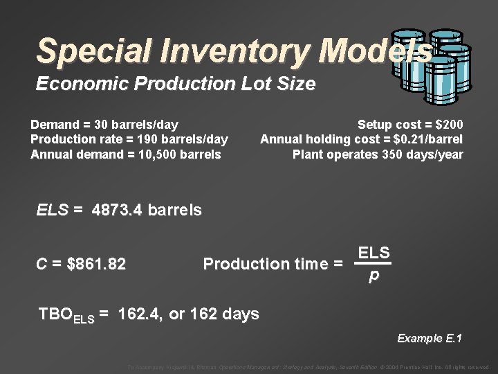
Special Inventory Models Economic Production Lot Size Demand = 30 barrels/day Production rate = 190 barrels/day Annual demand = 10, 500 barrels Setup cost = $200 Annual holding cost = $0. 21/barrel Plant operates 350 days/year ELS = 4873. 4 barrels C = $861. 82 ELS Production time = p TBOELS = 162. 4, or 162 days Example E. 1 To Accompany Krajewski & Ritzman Operations Management: Strategy and Analysis, Seventh Edition © 2004 Prentice Hall, Inc. All rights reserved.

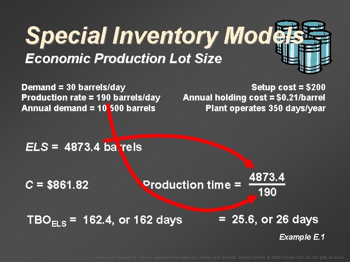
Special Inventory Models Economic Production Lot Size Demand = 30 barrels/day Production rate = 190 barrels/day Annual demand = 10, 500 barrels Setup cost = $200 Annual holding cost = $0. 21/barrel Plant operates 350 days/year ELS = 4873. 4 barrels C = $861. 82 4873. 4 Production time = 190 TBOELS = 162. 4, or 162 days = 25. 6, or 26 days Example E. 1 To Accompany Krajewski & Ritzman Operations Management: Strategy and Analysis, Seventh Edition © 2004 Prentice Hall, Inc. All rights reserved.

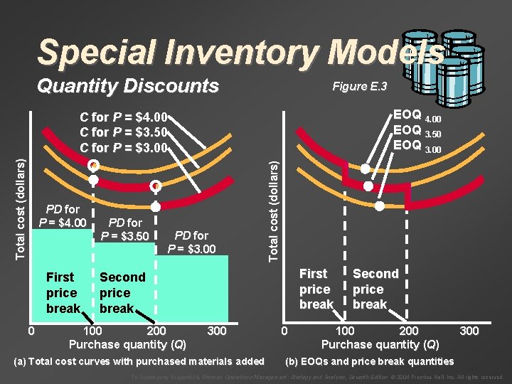
Special Inventory Models Quantity Discounts Figure E. 3 EOQ 4. 00 EOQ 3. 50 EOQ 3. 00 PD for P = $4. 00 First price break 0 PD for P = $3. 50 PD for P = $3. 00 Total cost (dollars) C for P = $4. 00 C for P = $3. 50 C for P = $3. 00 First price break Second price break 100 200 Purchase quantity (Q) 300 (a) Total cost curves with purchased materials added 0 Second price break 100 200 Purchase quantity (Q) 300 (b) EOQs and price break quantities To Accompany Krajewski & Ritzman Operations Management: Strategy and Analysis, Seventh Edition © 2004 Prentice Hall, Inc. All rights reserved.

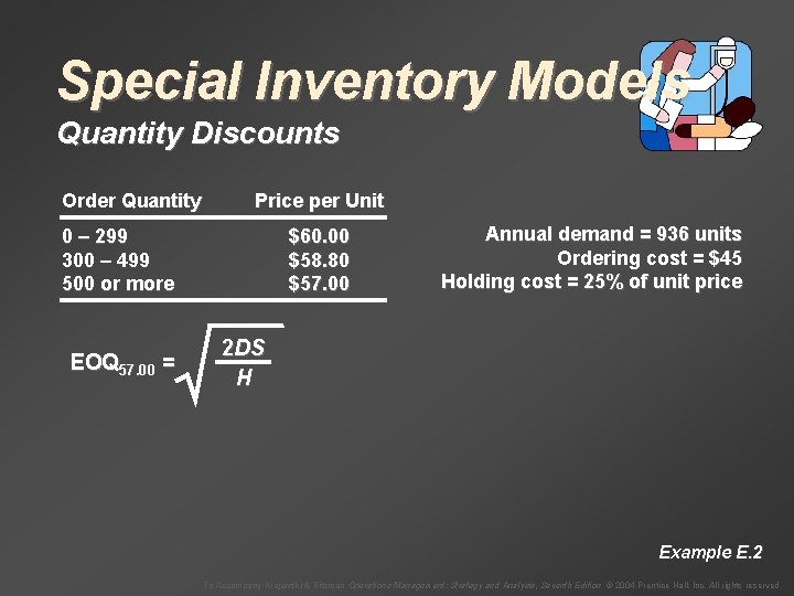
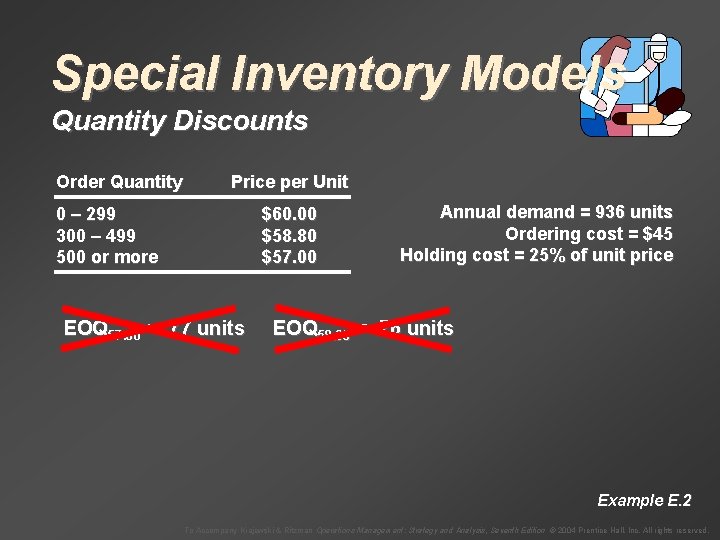
Special Inventory Models Quantity Discounts Order Quantity Price per Unit 0 – 299 300 – 499 500 or more EOQ 57. 00 = $60. 00 $58. 80 $57. 00 Annual demand = 936 units Ordering cost = $45 Holding cost = 25% of unit price 2 DS H Example E. 2 To Accompany Krajewski & Ritzman Operations Management: Strategy and Analysis, Seventh Edition © 2004 Prentice Hall, Inc. All rights reserved.

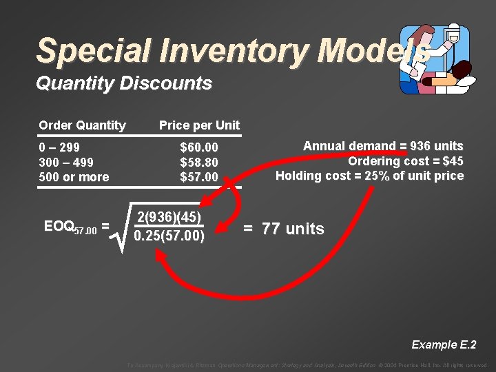
Special Inventory Models Quantity Discounts Order Quantity 0 – 299 300 – 499 500 or more EOQ 57. 00 = Price per Unit $60. 00 $58. 80 $57. 00 2(936)(45) 0. 25(57. 00) Annual demand = 936 units Ordering cost = $45 Holding cost = 25% of unit price = 77 units Example E. 2 To Accompany Krajewski & Ritzman Operations Management: Strategy and Analysis, Seventh Edition © 2004 Prentice Hall, Inc. All rights reserved.

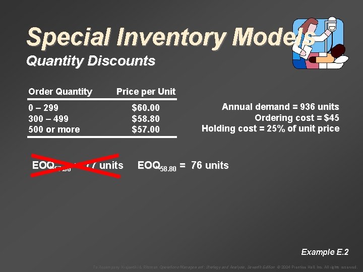
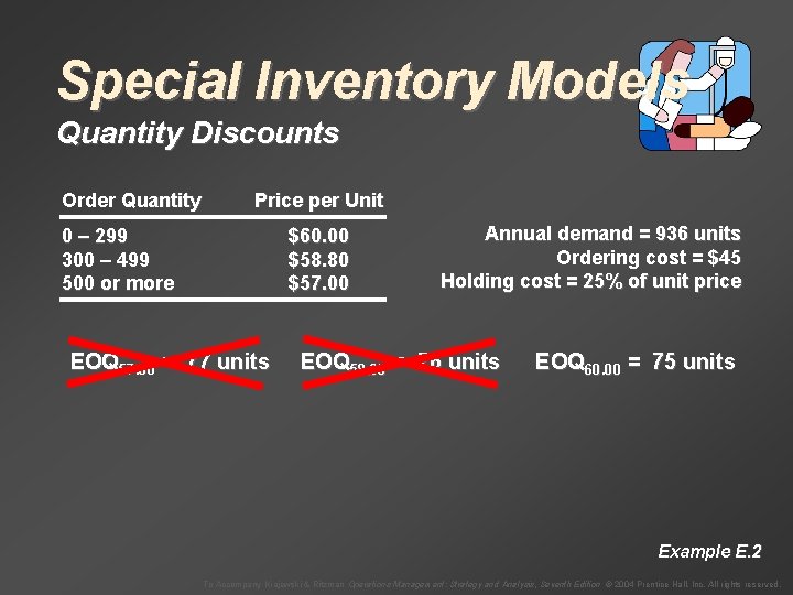
Special Inventory Models Quantity Discounts Order Quantity Price per Unit 0 – 299 300 – 499 500 or more $60. 00 $58. 80 $57. 00 EOQ 57. 00 = 77 units Annual demand = 936 units Ordering cost = $45 Holding cost = 25% of unit price EOQ 58. 80 = 76 units Example E. 2 To Accompany Krajewski & Ritzman Operations Management: Strategy and Analysis, Seventh Edition © 2004 Prentice Hall, Inc. All rights reserved.

Special Inventory Models Quantity Discounts Order Quantity Price per Unit 0 – 299 300 – 499 500 or more $60. 00 $58. 80 $57. 00 EOQ 57. 00 = 77 units Annual demand = 936 units Ordering cost = $45 Holding cost = 25% of unit price EOQ 58. 80 = 76 units EOQ 60. 00 = 75 units Example E. 2 To Accompany Krajewski & Ritzman Operations Management: Strategy and Analysis, Seventh Edition © 2004 Prentice Hall, Inc. All rights reserved.

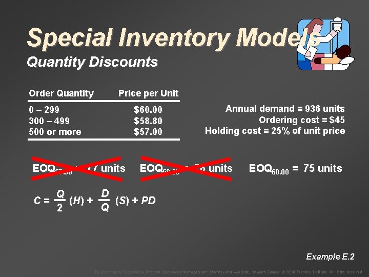
Special Inventory Models Quantity Discounts Order Quantity Price per Unit 0 – 299 300 – 499 500 or more $60. 00 $58. 80 $57. 00 EOQ 57. 00 = 77 units C= Annual demand = 936 units Ordering cost = $45 Holding cost = 25% of unit price EOQ 58. 80 = 76 units EOQ 60. 00 = 75 units D Q ( H) + (S) + PD Q 2 Example E. 2 To Accompany Krajewski & Ritzman Operations Management: Strategy and Analysis, Seventh Edition © 2004 Prentice Hall, Inc. All rights reserved.

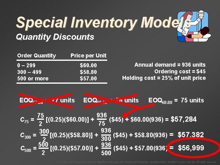
Special Inventory Models Quantity Discounts Order Quantity Price per Unit 0 – 299 300 – 499 500 or more $60. 00 $58. 80 $57. 00 EOQ 57. 00 = 77 units Annual demand = 936 units Ordering cost = $45 Holding cost = 25% of unit price EOQ 58. 80 = 76 units EOQ 60. 00 = 75 units 936 75 [(0. 25)($60. 00)] + ($45) + $60. 00(936) = $57, 284 75 2 936 300 C 300 = [(0. 25)($58. 80)] + ($45) + $58. 80(936) = $57, 382 300 2 500 936 C 500 = [(0. 25)($57. 00)] + ($45) + $57. 00(936) = $56, 999 2 500 C 75 = To Accompany Krajewski & Ritzman Operations Management: Strategy and Analysis, Seventh Edition © 2004 Prentice Hall, Inc. All rights reserved.

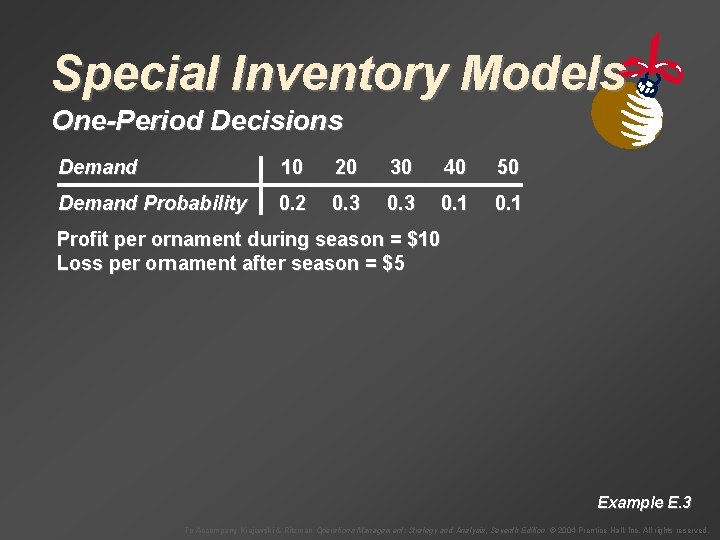
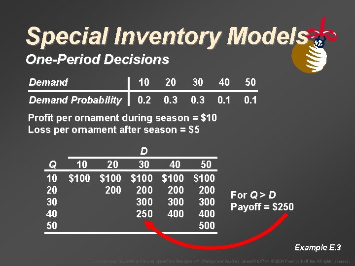
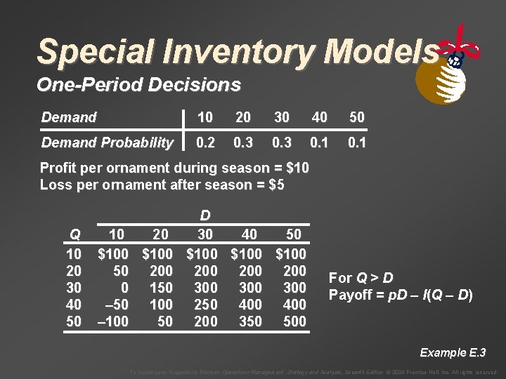
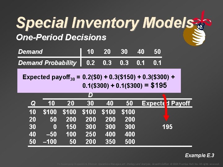
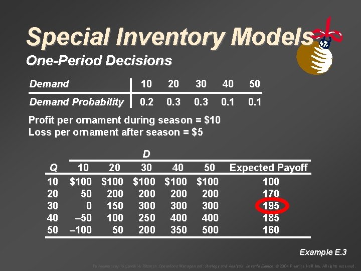
Special Inventory Models One-Period Decisions Demand 10 20 30 40 50 Demand Probability 0. 2 0. 3 0. 1 Profit per ornament during season = $10 Loss per ornament after season = $5 Example E. 3 To Accompany Krajewski & Ritzman Operations Management: Strategy and Analysis, Seventh Edition © 2004 Prentice Hall, Inc. All rights reserved.

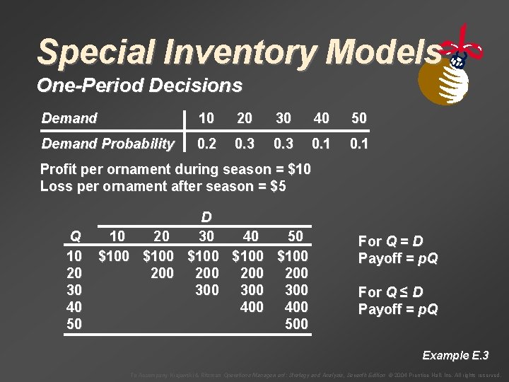
Special Inventory Models One-Period Decisions Demand 10 20 30 40 50 Demand Probability 0. 2 0. 3 0. 1 Profit per ornament during season = $10 Loss per ornament after season = $5 Q 10 20 30 40 50 D 10 20 30 40 50 $100 $100 200 200 300 300 400 500 For Q = D Payoff = p. Q For Q ≤ D Payoff = p. Q Example E. 3 To Accompany Krajewski & Ritzman Operations Management: Strategy and Analysis, Seventh Edition © 2004 Prentice Hall, Inc. All rights reserved.

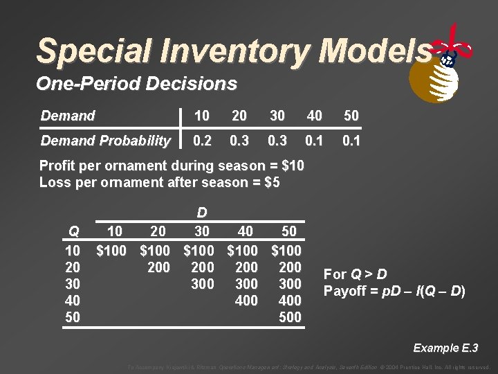
Special Inventory Models One-Period Decisions Demand 10 20 30 40 50 Demand Probability 0. 2 0. 3 0. 1 Profit per ornament during season = $10 Loss per ornament after season = $5 Q 10 20 30 40 50 D 10 20 30 40 50 $100 $100 200 200 300 300 400 500 For Q > D Payoff = p. D – I(Q – D) Example E. 3 To Accompany Krajewski & Ritzman Operations Management: Strategy and Analysis, Seventh Edition © 2004 Prentice Hall, Inc. All rights reserved.

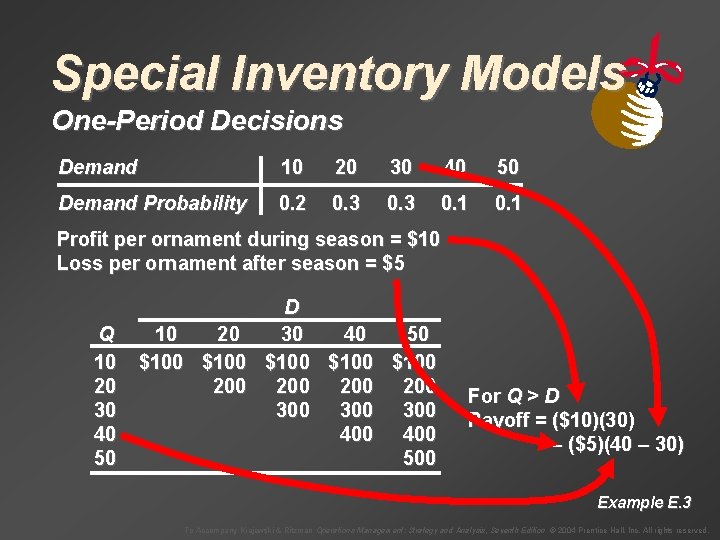
Special Inventory Models One-Period Decisions Demand 10 20 30 40 50 Demand Probability 0. 2 0. 3 0. 1 Profit per ornament during season = $10 Loss per ornament after season = $5 Q 10 20 30 40 50 D 10 20 30 40 50 $100 $100 200 200 300 300 400 500 For Q > D Payoff = ($10)(30) – ($5)(40 – 30) Example E. 3 To Accompany Krajewski & Ritzman Operations Management: Strategy and Analysis, Seventh Edition © 2004 Prentice Hall, Inc. All rights reserved.

Special Inventory Models One-Period Decisions Demand 10 20 30 40 50 Demand Probability 0. 2 0. 3 0. 1 Profit per ornament during season = $10 Loss per ornament after season = $5 Q 10 20 30 40 50 D 10 20 30 40 50 $100 $100 200 200 300 300 250 400 500 For Q > D Payoff = $250 Example E. 3 To Accompany Krajewski & Ritzman Operations Management: Strategy and Analysis, Seventh Edition © 2004 Prentice Hall, Inc. All rights reserved.

Special Inventory Models One-Period Decisions Demand 10 20 30 40 50 Demand Probability 0. 2 0. 3 0. 1 Profit per ornament during season = $10 Loss per ornament after season = $5 Q 10 20 30 40 50 10 20 $100 50 200 0 150 – 50 100 – 100 50 D 30 40 50 $100 200 200 300 300 250 400 200 350 500 For Q > D Payoff = p. D – I(Q – D) Example E. 3 To Accompany Krajewski & Ritzman Operations Management: Strategy and Analysis, Seventh Edition © 2004 Prentice Hall, Inc. All rights reserved.

Special Inventory Models One-Period Decisions Demand 10 20 30 40 50 Demand Probability 0. 2 0. 3 0. 1 Profit per ornament during season = $10 Expected payoff = 0. 2($0) + 0. 3($150) + 0. 3($300) + Loss per ornament 30 after season = $5 0. 1($300) + 0. 1($300) = $195 D Q 10 20 30 40 50 Expected Payoff 10 $100 $100 20 50 200 200 30 0 150 300 300 195 40 – 50 100 250 400 50 – 100 50 200 350 500 Example E. 3 To Accompany Krajewski & Ritzman Operations Management: Strategy and Analysis, Seventh Edition © 2004 Prentice Hall, Inc. All rights reserved.

Special Inventory Models One-Period Decisions Demand 10 20 30 40 50 Demand Probability 0. 2 0. 3 0. 1 Profit per ornament during season = $10 Loss per ornament after season = $5 Q 10 20 30 40 50 10 20 $100 50 200 0 150 – 50 100 – 100 50 D 30 40 50 $100 200 200 300 300 250 400 200 350 500 Expected Payoff 100 170 195 185 160 Example E. 3 To Accompany Krajewski & Ritzman Operations Management: Strategy and Analysis, Seventh Edition © 2004 Prentice Hall, Inc. All rights reserved.