Inventory Management Chapter 12 2007 Pearson Education Inventory

Inventory Management Chapter 12 © 2007 Pearson Education

Inventory Management Ø Inventory management is the planning and controlling of inventories in order to meet the competitive priorities of the organization. Ø Effective inventory management is essential for realizing the full potential of any value chain. Ø Inventory management requires information about expected demands, amounts on hand amounts on order for every item stocked at all locations. Ø The appropriate timing and size of the reorder quantities must also be determined. © 2007 Pearson Education

Inventory Basics Ø Inventory is created when the receipt of materials, parts, or finished goods exceeds their disbursement. Ø Inventory is depleted when their disbursement exceeds their receipt. Ø An inventory manager’s job is to balance the advantages and disadvantages of both low and high inventories. Ø Both have associated cost characteristics. © 2007 Pearson Education

Pressures for Low Inventories Ø Inventory holding cost is the sum of the cost of capital and the variable costs of keeping items on hand, such as storage and handling, taxes, insurance, and shrinkage. Ø Cost of Capital is the opportunity cost of investing in an asset relative to the expected return on assets of similar risk. Ø Storage and Handling arise from moving in and out of a storage facility plus the rental cost and/or opportunity cost of that space. Ø Taxes, Insurance, and Shrinkage: More taxes are paid and insurance costs are higher if end-of-the-year inventories are high. Shrinkage comes from theft, obsolescence and deterioration. © 2007 Pearson Education

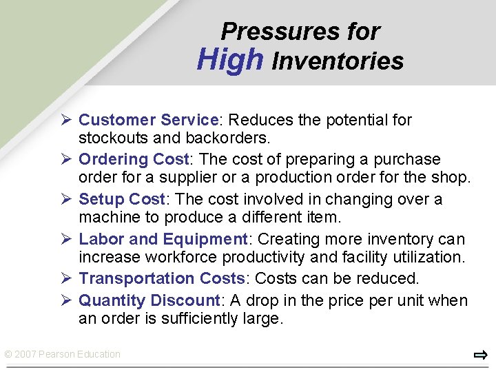
Pressures for High Inventories Ø Customer Service: Reduces the potential for stockouts and backorders. Ø Ordering Cost: The cost of preparing a purchase order for a supplier or a production order for the shop. Ø Setup Cost: The cost involved in changing over a machine to produce a different item. Ø Labor and Equipment: Creating more inventory can increase workforce productivity and facility utilization. Ø Transportation Costs: Costs can be reduced. Ø Quantity Discount: A drop in the price per unit when an order is sufficiently large. © 2007 Pearson Education

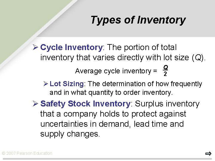
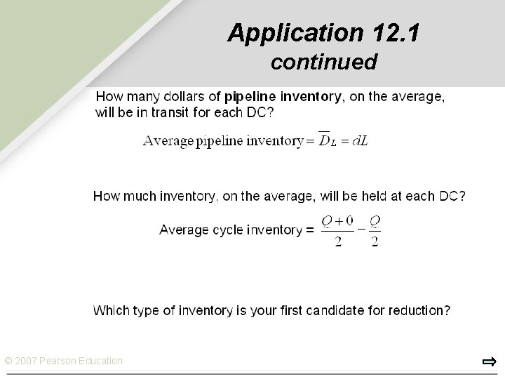
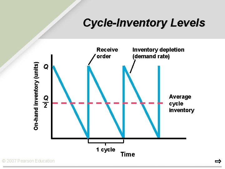
Types of Inventory Ø Cycle Inventory: The portion of total inventory that varies directly with lot size (Q). Q Average cycle inventory = 2 Ø Lot Sizing: The determination of how frequently and in what quantity to order inventory. Ø Safety Stock Inventory: Surplus inventory that a company holds to protect against uncertainties in demand, lead time and supply changes. © 2007 Pearson Education

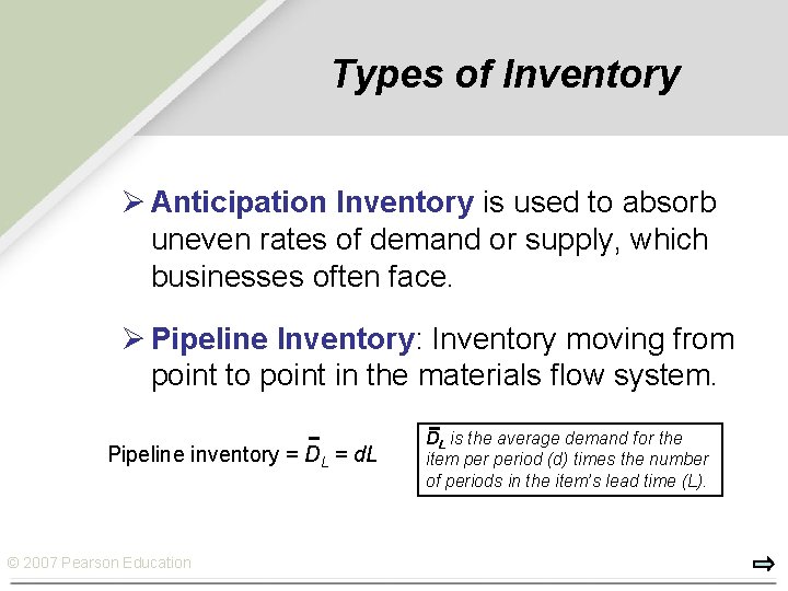
Types of Inventory Ø Anticipation Inventory is used to absorb uneven rates of demand or supply, which businesses often face. Ø Pipeline Inventory: Inventory moving from point to point in the materials flow system. Pipeline inventory = DL = d. L © 2007 Pearson Education DL is the average demand for the item period (d) times the number of periods in the item’s lead time (L).

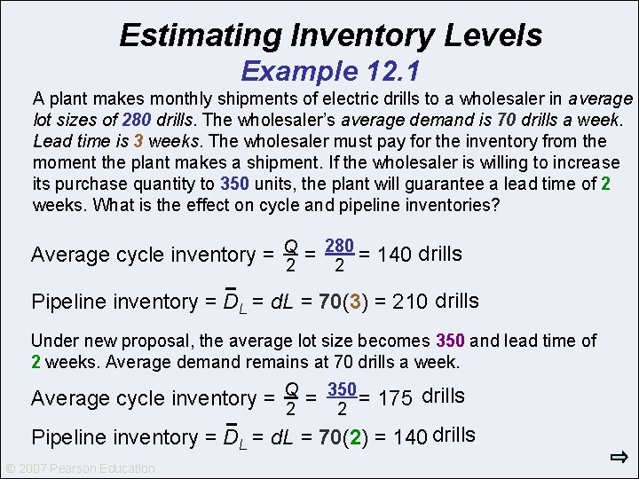
Estimating Inventory Levels Example 12. 1 A plant makes monthly shipments of electric drills to a wholesaler in average lot sizes of 280 drills. The wholesaler’s average demand is 70 drills a week. Lead time is 3 weeks. The wholesaler must pay for the inventory from the moment the plant makes a shipment. If the wholesaler is willing to increase its purchase quantity to 350 units, the plant will guarantee a lead time of 2 weeks. What is the effect on cycle and pipeline inventories? 280 Average cycle inventory = Q = = 140 drills 2 2 Pipeline inventory = DL = d. L = 70(3) = 210 drills Under new proposal, the average lot size becomes 350 and lead time of 2 weeks. Average demand remains at 70 drills a week. 350 Average cycle inventory = Q = = 175 drills 2 2 Pipeline inventory = DL = d. L = 70(2) = 140 drills © 2007 Pearson Education

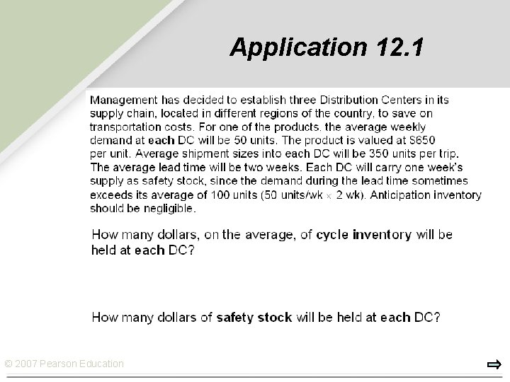
Application 12. 1 © 2007 Pearson Education

Application 12. 1 continued © 2007 Pearson Education

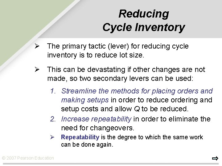
Reducing Cycle Inventory Ø The primary tactic (lever) for reducing cycle inventory is to reduce lot size. Ø This can be devastating if other changes are not made, so two secondary levers can be used: 1. Streamline the methods for placing orders and making setups in order to reduce ordering and setup costs and allow Q to be reduced. 2. Increase repeatability in order to eliminate the need for changeovers. Ø Repeatability is the degree to which the same work can be done again. © 2007 Pearson Education

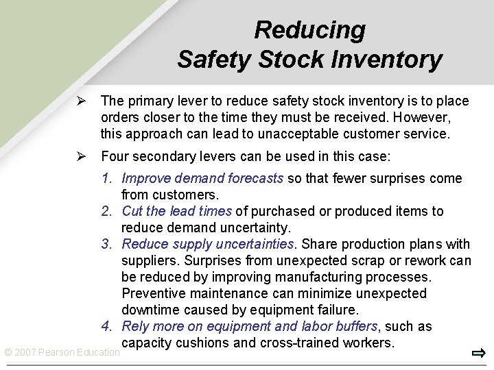
Reducing Safety Stock Inventory Ø The primary lever to reduce safety stock inventory is to place orders closer to the time they must be received. However, this approach can lead to unacceptable customer service. Ø Four secondary levers can be used in this case: 1. Improve demand forecasts so that fewer surprises come from customers. 2. Cut the lead times of purchased or produced items to reduce demand uncertainty. 3. Reduce supply uncertainties. Share production plans with suppliers. Surprises from unexpected scrap or rework can be reduced by improving manufacturing processes. Preventive maintenance can minimize unexpected downtime caused by equipment failure. 4. Rely more on equipment and labor buffers, such as capacity cushions and cross-trained workers. © 2007 Pearson Education

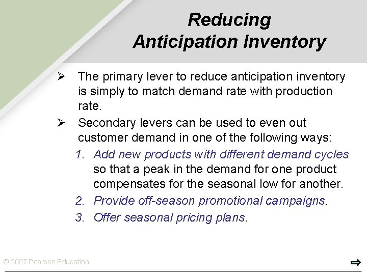
Reducing Anticipation Inventory Ø The primary lever to reduce anticipation inventory is simply to match demand rate with production rate. Ø Secondary levers can be used to even out customer demand in one of the following ways: 1. Add new products with different demand cycles so that a peak in the demand for one product compensates for the seasonal low for another. 2. Provide off-season promotional campaigns. 3. Offer seasonal pricing plans. © 2007 Pearson Education

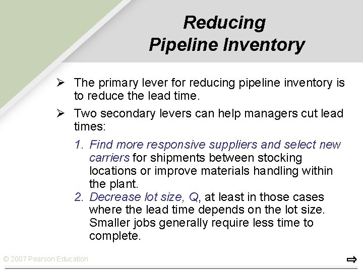
Reducing Pipeline Inventory Ø The primary lever for reducing pipeline inventory is to reduce the lead time. Ø Two secondary levers can help managers cut lead times: 1. Find more responsive suppliers and select new carriers for shipments between stocking locations or improve materials handling within the plant. 2. Decrease lot size, Q, at least in those cases where the lead time depends on the lot size. Smaller jobs generally require less time to complete. © 2007 Pearson Education

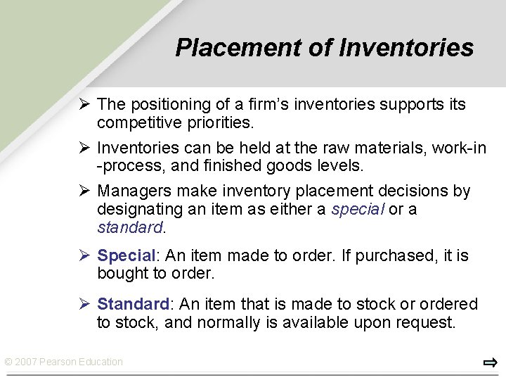
Placement of Inventories Ø The positioning of a firm’s inventories supports its competitive priorities. Ø Inventories can be held at the raw materials, work-in -process, and finished goods levels. Ø Managers make inventory placement decisions by designating an item as either a special or a standard. Ø Special: An item made to order. If purchased, it is bought to order. Ø Standard: An item that is made to stock or ordered to stock, and normally is available upon request. © 2007 Pearson Education

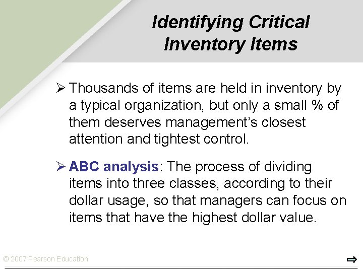
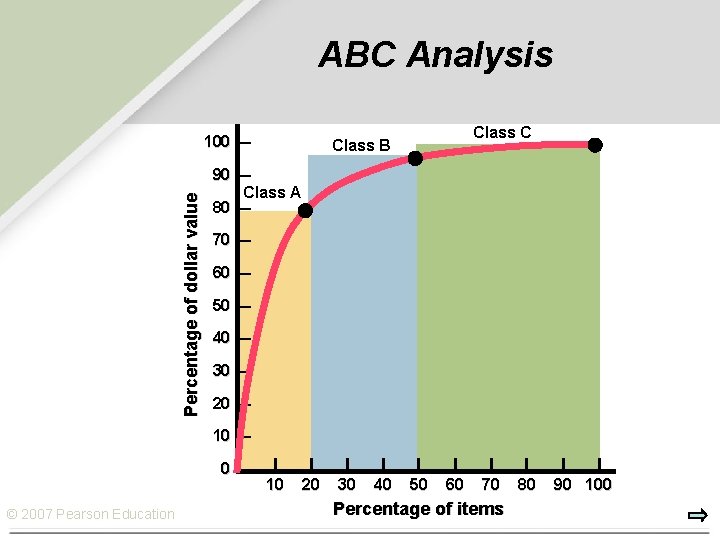
Identifying Critical Inventory Items Ø Thousands of items are held in inventory by a typical organization, but only a small % of them deserves management’s closest attention and tightest control. Ø ABC analysis: The process of dividing items into three classes, according to their dollar usage, so that managers can focus on items that have the highest dollar value. © 2007 Pearson Education

ABC Analysis Percentage of dollar value 100 — Class C Class B 90 — Class A 80 — 70 — 60 — 50 — 40 — 30 — 20 — 10 — 0— © 2007 Pearson Education 10 20 30 40 50 60 70 Percentage of items 80 90 100

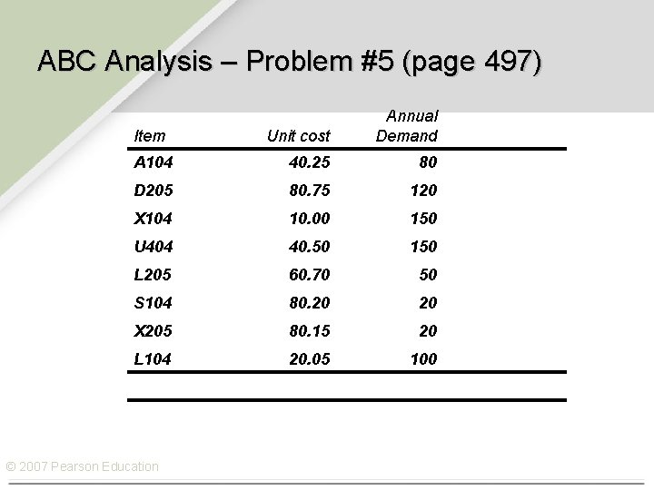
ABC Analysis – Problem #5 (page 497) Item Annual Demand Unit cost A 104 40. 25 D 205 80. 75 120 X 104 10. 00 150 U 404 40. 50 150 L 205 60. 70 50 S 104 80. 20 20 X 205 80. 15 20 L 104 20. 05 100 © 2007 Pearson Education 80

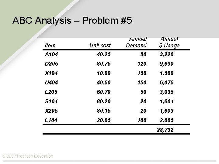
ABC Analysis – Problem #5 Item Annual Demand Unit cost Annual $ Usage A 104 40. 25 80 3, 220 D 205 80. 75 120 9, 690 X 104 10. 00 150 1, 500 U 404 40. 50 150 6, 075 L 205 60. 70 50 3, 035 S 104 80. 20 20 1, 604 X 205 80. 15 20 1, 603 L 104 20. 05 100 2, 005 © 2007 Pearson Education 28, 732

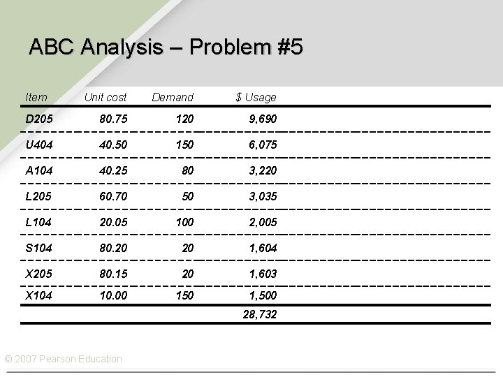
ABC Analysis – Problem #5 Item Unit cost Demand $ Usage D 205 80. 75 120 9, 690 U 404 40. 50 150 6, 075 A 104 40. 25 80 3, 220 L 205 60. 70 50 3, 035 L 104 20. 05 100 2, 005 S 104 80. 20 20 1, 604 X 205 80. 15 20 1, 603 X 104 10. 00 150 1, 500 © 2007 Pearson Education 28, 732

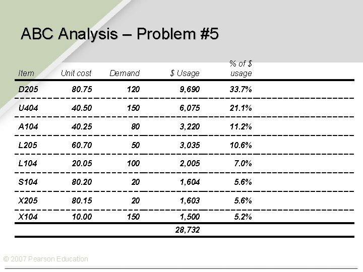
ABC Analysis – Problem #5 Unit cost Demand $ Usage % of $ usage D 205 80. 75 120 9, 690 33. 7% U 404 40. 50 150 6, 075 21. 1% A 104 40. 25 80 3, 220 11. 2% L 205 60. 70 50 3, 035 10. 6% L 104 20. 05 100 2, 005 7. 0% S 104 80. 20 20 1, 604 5. 6% X 205 80. 15 20 1, 603 5. 6% X 104 10. 00 150 1, 500 5. 2% Item © 2007 Pearson Education 28, 732

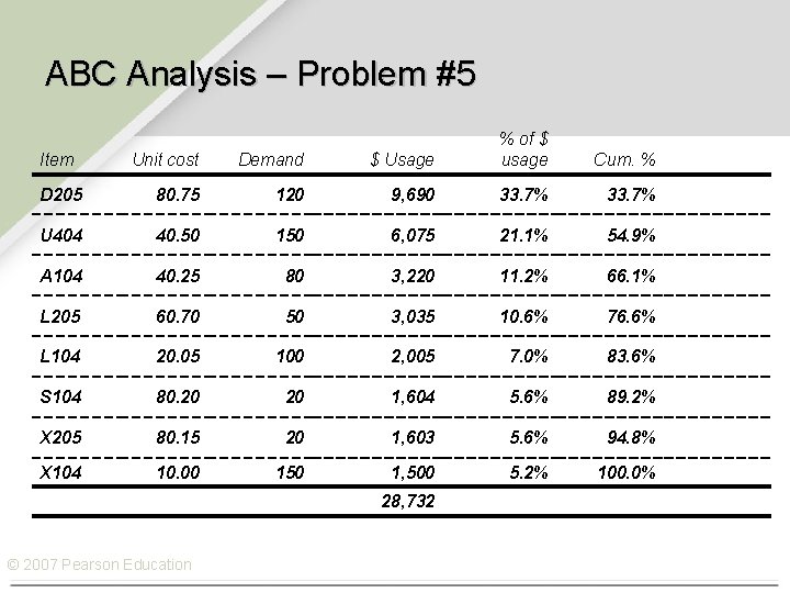
ABC Analysis – Problem #5 Unit cost Demand $ Usage % of $ usage D 205 80. 75 120 9, 690 33. 7% U 404 40. 50 150 6, 075 21. 1% 54. 9% A 104 40. 25 80 3, 220 11. 2% 66. 1% L 205 60. 70 50 3, 035 10. 6% 76. 6% L 104 20. 05 100 2, 005 7. 0% 83. 6% S 104 80. 20 20 1, 604 5. 6% 89. 2% X 205 80. 15 20 1, 603 5. 6% 94. 8% X 104 10. 00 150 1, 500 5. 2% 100. 0% Item © 2007 Pearson Education 28, 732 Cum. %

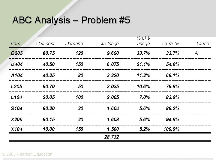
ABC Analysis – Problem #5 Unit cost Demand $ Usage % of $ usage D 205 80. 75 120 9, 690 33. 7% U 404 40. 50 150 6, 075 21. 1% 54. 9% A 104 40. 25 80 3, 220 11. 2% 66. 1% L 205 60. 70 50 3, 035 10. 6% 76. 6% L 104 20. 05 100 2, 005 7. 0% 83. 6% S 104 80. 20 20 1, 604 5. 6% 89. 2% X 205 80. 15 20 1, 603 5. 6% 94. 8% X 104 10. 00 150 1, 500 5. 2% 100. 0% Item © 2007 Pearson Education 28, 732 Cum. % Class A

ABC Analysis – Problem #5 Unit cost Demand $ Usage % of $ usage D 205 80. 75 120 9, 690 33. 7% U 404 40. 50 150 6, 075 21. 1% 54. 9% A 104 40. 25 80 3, 220 11. 2% 66. 1% L 205 60. 70 50 3, 035 10. 6% 76. 6% L 104 20. 05 100 2, 005 7. 0% 83. 6% C S 104 80. 20 20 1, 604 5. 6% 89. 2% C X 205 80. 15 20 1, 603 5. 6% 94. 8% C X 104 10. 00 150 1, 500 5. 2% 100. 0% C Item © 2007 Pearson Education 28, 732 Cum. % Class A

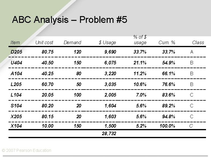
ABC Analysis – Problem #5 Unit cost Demand $ Usage % of $ usage D 205 80. 75 120 9, 690 33. 7% A U 404 40. 50 150 6, 075 21. 1% 54. 9% B A 104 40. 25 80 3, 220 11. 2% 66. 1% B L 205 60. 70 50 3, 035 10. 6% 76. 6% B L 104 20. 05 100 2, 005 7. 0% 83. 6% C S 104 80. 20 20 1, 604 5. 6% 89. 2% C X 205 80. 15 20 1, 603 5. 6% 94. 8% C X 104 10. 00 150 1, 500 5. 2% 100. 0% C Item © 2007 Pearson Education 28, 732 Cum. % Class

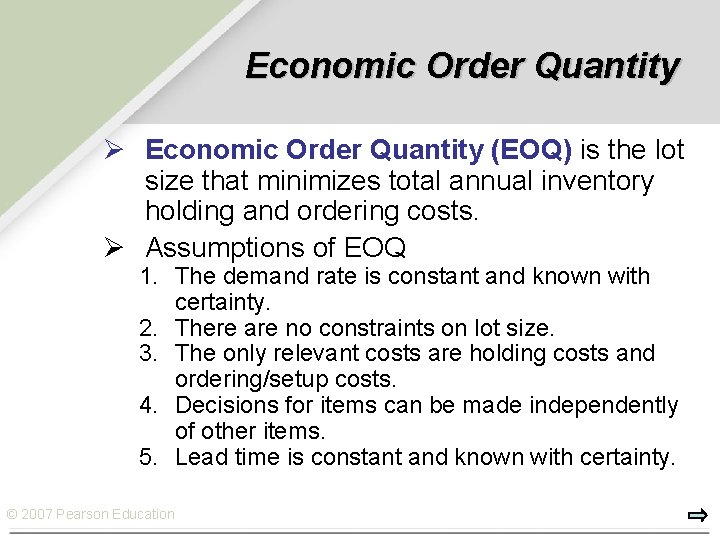
Economic Order Quantity Ø Economic Order Quantity (EOQ) is the lot size that minimizes total annual inventory holding and ordering costs. Ø Assumptions of EOQ 1. The demand rate is constant and known with certainty. 2. There are no constraints on lot size. 3. The only relevant costs are holding costs and ordering/setup costs. 4. Decisions for items can be made independently of other items. 5. Lead time is constant and known with certainty. © 2007 Pearson Education

Cycle-Inventory Levels On-hand inventory (units) Receive order Inventory depletion (demand rate) Q Average cycle inventory Q — 2 1 cycle © 2007 Pearson Education Time

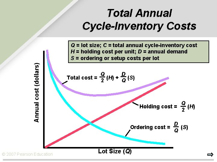
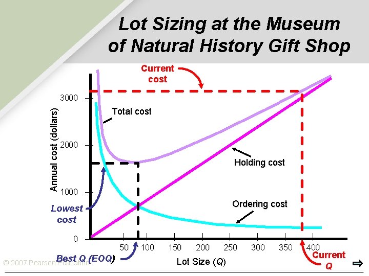
Total Annual Cycle-Inventory Costs Annual cost (dollars) Q = lot size; C = total annual cycle-inventory cost H = holding cost per unit; D = annual demand S = ordering or setup costs per lot Q D Total cost = ( H) + ( S) 2 Q Holding cost = Ordering cost = © 2007 Pearson Education Lot Size (Q) Q ( H) 2 D ( S) Q

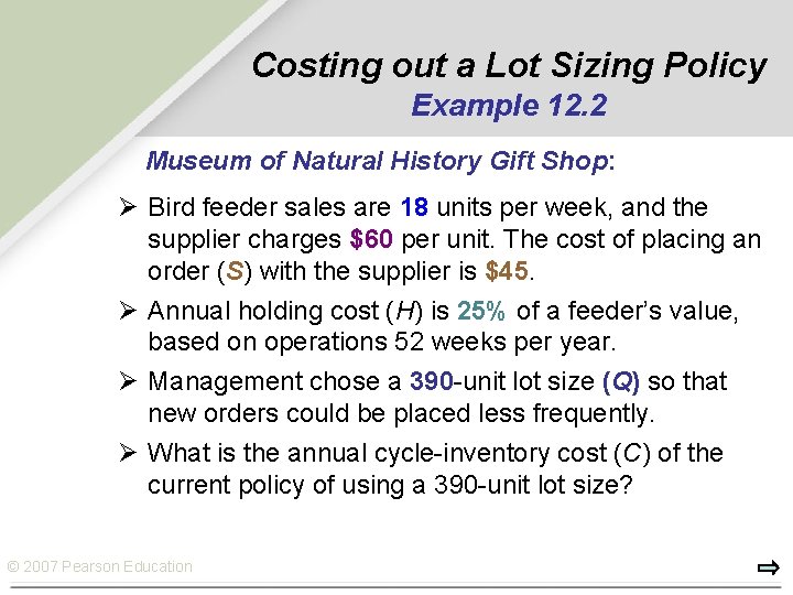
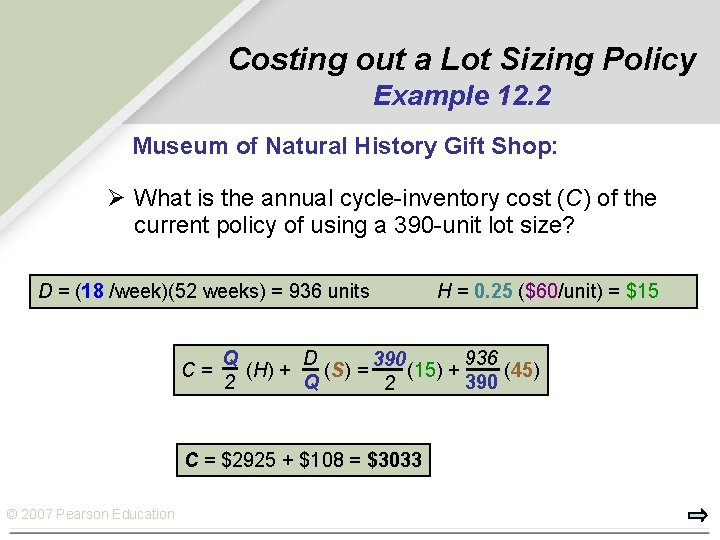
Costing out a Lot Sizing Policy Example 12. 2 Museum of Natural History Gift Shop: Ø Bird feeder sales are 18 units per week, and the supplier charges $60 per unit. The cost of placing an order (S) with the supplier is $45. Ø Annual holding cost (H) is 25% of a feeder’s value, based on operations 52 weeks per year. Ø Management chose a 390 -unit lot size (Q) so that new orders could be placed less frequently. Ø What is the annual cycle-inventory cost (C) of the current policy of using a 390 -unit lot size? © 2007 Pearson Education

Costing out a Lot Sizing Policy Example 12. 2 Museum of Natural History Gift Shop: Ø What is the annual cycle-inventory cost (C) of the current policy of using a 390 -unit lot size? D = (18 /week)(52 weeks) = 936 units C= Q D 936 390 (H) + (S) = (15) + (45) 2 Q 390 2 C = $2925 + $108 = $3033 © 2007 Pearson Education H = 0. 25 ($60/unit) = $15

Lot Sizing at the Museum of Natural History Gift Shop Current cost Annual cost (dollars) 3000 — Total cost 2000 — Holding cost 1000 — Ordering cost Lowest cost 0 — © 2007 Pearson Best Q (EOQ) Education | 50 | 100 | 150 | 200 | 250 Lot Size (Q) | 300 | 350 | 400 Current Q

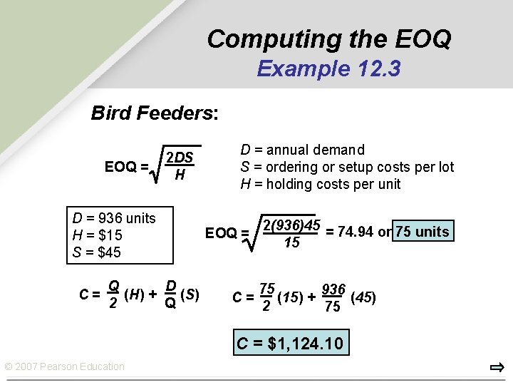
Computing the EOQ Example 12. 3 Bird Feeders: EOQ = 2 DS H D = 936 units H = $15 S = $45 C= Q D (H) + (S) 2 Q D = annual demand S = ordering or setup costs per lot H = holding costs per unit EOQ = C= 2(936)45 = 74. 94 or 75 units 15 75 936 (15) + (45) 2 75 C = $1, 124. 10 © 2007 Pearson Education

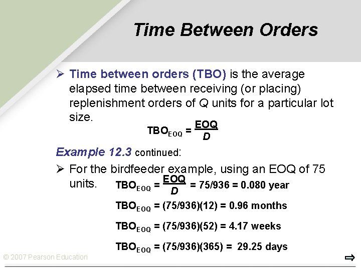
Time Between Orders Ø Time between orders (TBO) is the average elapsed time between receiving (or placing) replenishment orders of Q units for a particular lot size. EOQ TBOEOQ = D Example 12. 3 continued: Ø For the birdfeeder example, using an EOQ of 75 units. TBOEOQ = 75/936 = 0. 080 year D TBOEOQ = (75/936)(12) = 0. 96 months TBOEOQ = (75/936)(52) = 4. 17 weeks © 2007 Pearson Education TBOEOQ = (75/936)(365) = 29. 25 days

Understanding the Effect of Changes Ø A Change in the Demand Rate (D): When demand rises, the lot size also rises, but more slowly than actual demand. Ø A Change in the Setup Costs (S): Increasing S increases the EOQ and, consequently, the average cycle inventory. Ø A Change in the Holding Costs (H): EOQ declines when H increases. Ø Errors in Estimating D, H, and S: Total cost is fairly insensitive to errors, even when the estimates are wrong by a large margin. The reasons are that errors tend to cancel each other out and that the square root reduces the effect of the error. © 2007 Pearson Education

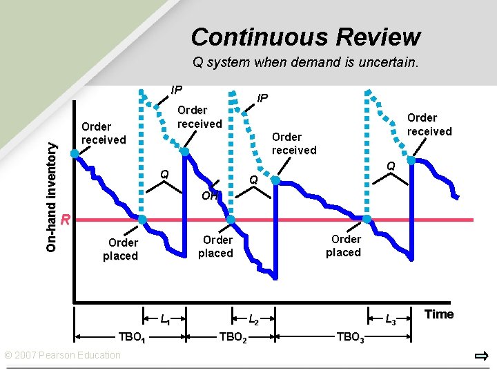
Inventory Control Systems Ø Inventory control systems tell us how much to order and when to place the order. Ø Independent demand items: Items for which demand is influenced by market conditions and is not related to the inventory decisions for any other item held in stock. Ø Continuous review (Q) systems (Reorder point systems ROP) are designed to track the remaining inventory of an item each time a withdrawal is made to determine whether it is time to reorder. Ø Periodic review (P) systems (Fixed Interval Reorder systems) in which an item’s inventory position is reviewed periodically rather than continuously. © 2007 Pearson Education

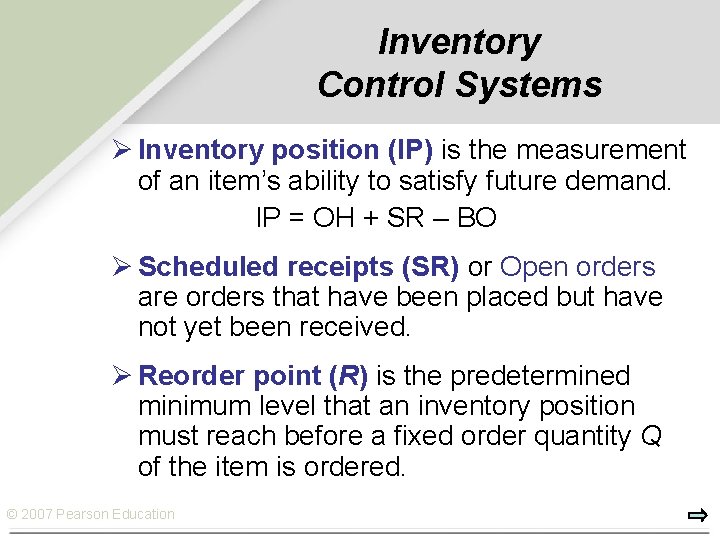
Inventory Control Systems Ø Inventory position (IP) is the measurement of an item’s ability to satisfy future demand. IP = OH + SR – BO Ø Scheduled receipts (SR) or Open orders are orders that have been placed but have not yet been received. Ø Reorder point (R) is the predetermined minimum level that an inventory position must reach before a fixed order quantity Q of the item is ordered. © 2007 Pearson Education

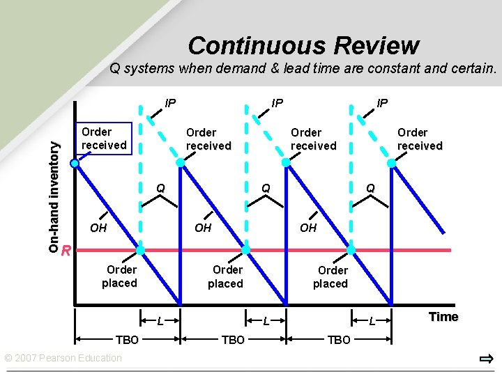
Continuous Review Q systems when demand & lead time are constant and certain. IP On-hand inventory IP Order received Q Q OH OH IP Q OH R Order placed L TBO © 2007 Pearson Education Order placed L TBO Time

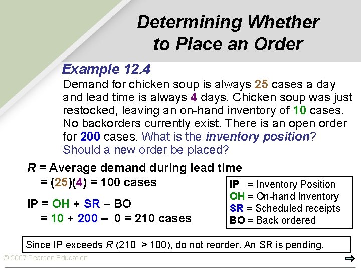
Determining Whether to Place an Order Example 12. 4 Demand for chicken soup is always 25 cases a day and lead time is always 4 days. Chicken soup was just restocked, leaving an on-hand inventory of 10 cases. No backorders currently exist. There is an open order for 200 cases. What is the inventory position? Should a new order be placed? R = Average demand during lead time = (25)(4) = 100 cases IP = Inventory Position IP = OH + SR – BO = 10 + 200 – 0 = 210 cases OH = On-hand Inventory SR = Scheduled receipts BO = Back ordered Since IP exceeds R (210 > 100), do not reorder. An SR is pending. © 2007 Pearson Education

Continuous Review Q system when demand is uncertain. On-hand inventory IP Order received Q Q Q OH R L 1 TBO 1 © 2007 Pearson Education Order placed L 2 TBO 2 L 3 TBO 3 Time

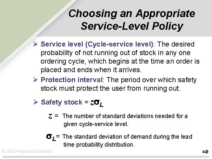
Choosing an Appropriate Service-Level Policy Ø Service level (Cycle-service level): The desired probability of not running out of stock in any one ordering cycle, which begins at the time an order is placed and ends when it arrives. Ø Protection interval: The period over which safety stock must protect the user from running out. Ø Safety stock = z L z= The number of standard deviations needed for a given cycle-service level. L= The standard deviation of demand during the lead time probability distribution. © 2007 Pearson Education

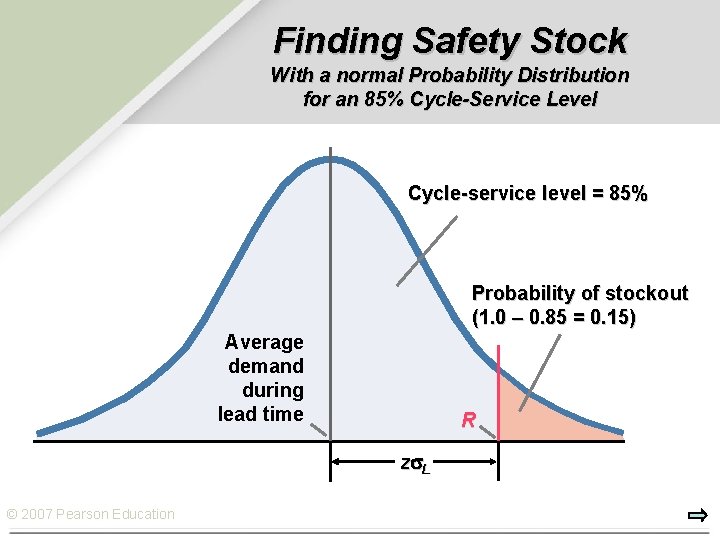
Finding Safety Stock With a normal Probability Distribution for an 85% Cycle-Service Level Cycle-service level = 85% Probability of stockout (1. 0 – 0. 85 = 0. 15) Average demand during lead time R z L © 2007 Pearson Education

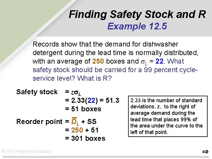
Finding Safety Stock and R Example 12. 5 Records show that the demand for dishwasher detergent during the lead time is normally distributed, with an average of 250 boxes and L = 22. What safety stock should be carried for a 99 percent cycleservice level? What is R? Safety stock = z L = 2. 33(22) = 51. 3 = 51 boxes Reorder point = DL + SS = 250 + 51 = 301 boxes © 2007 Pearson Education 2. 33 is the number of standard deviations, z, to the right of average demand during the lead time that places 99% of the area under the curve to the left of that point.

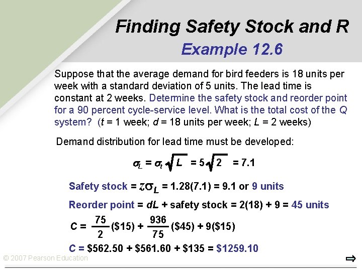
Finding Safety Stock and R Example 12. 6 Suppose that the average demand for bird feeders is 18 units per week with a standard deviation of 5 units. The lead time is constant at 2 weeks. Determine the safety stock and reorder point for a 90 percent cycle-service level. What is the total cost of the Q system? (t = 1 week; d = 18 units per week; L = 2 weeks) Demand distribution for lead time must be developed: s. L = st L = 5 2 = 7. 1 Safety stock = z L = 1. 28(7. 1) = 9. 1 or 9 units Reorder point = d. L + safety stock = 2(18) + 9 = 45 units 75 936 C = ($15) + ($45) + 9($15) 2 75 C = $562. 50 + $561. 60 + $135 = $1259. 10 © 2007 Pearson Education

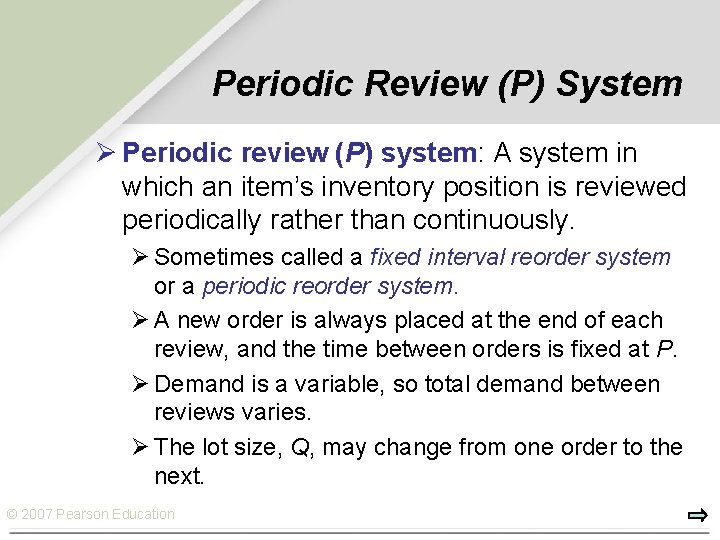
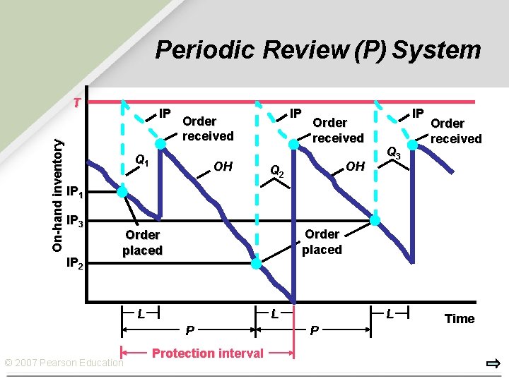
Periodic Review (P) System Ø Periodic review (P) system: A system in which an item’s inventory position is reviewed periodically rather than continuously. Ø Sometimes called a fixed interval reorder system or a periodic reorder system. Ø A new order is always placed at the end of each review, and the time between orders is fixed at P. Ø Demand is a variable, so total demand between reviews varies. Ø The lot size, Q, may change from one order to the next. © 2007 Pearson Education

Periodic Review (P) System On-hand inventory T IP IP Order received Q 1 OH Order received OH Q 2 IP Q 3 Order received IP 1 IP 3 IP 2 Order placed L L P © 2007 Pearson Education Protection interval L P Time

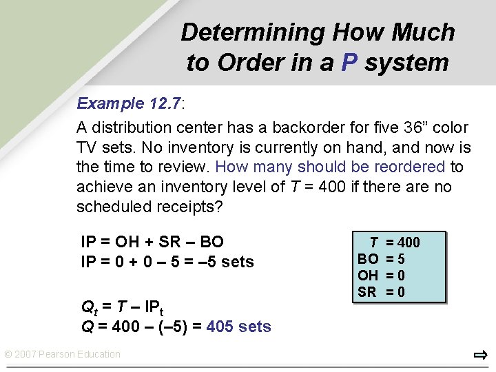
Determining How Much to Order in a P system Example 12. 7: A distribution center has a backorder for five 36” color TV sets. No inventory is currently on hand, and now is the time to review. How many should be reordered to achieve an inventory level of T = 400 if there are no scheduled receipts? IP = OH + SR – BO IP = 0 + 0 – 5 = – 5 sets Qt = T – IPt Q = 400 – (– 5) = 405 sets © 2007 Pearson Education T BO OH SR = 400 =5 =0 =0

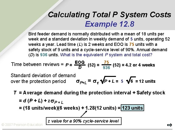
Calculating Total P System Costs Example 12. 8 Bird feeder demand is normally distributed with a mean of 18 units per week and a standard deviation in weekly demand of 5 units, operating 52 weeks a year. Lead time (L) is 2 weeks and EOQ is 75 units with a safety stock of 9 units and a cycle-service level of 90%. Annual demand (D) is 936 units. What is the equivalent P system and total cost? Time between reviews = P = EOQ (52) = 75 (52) = 4. 2 or 4 weeks D Standard deviation of demand P+L = over the protection period 936 t P + L = 5 6 = 12 units T = Average demand during the protection interval + Safety stock = d (P + L) + z P + L = (18 units/week)(6 weeks) + 1. 28(12 units) = 123 units © 2007 Pearson Education z value for a 90% cycle-service level

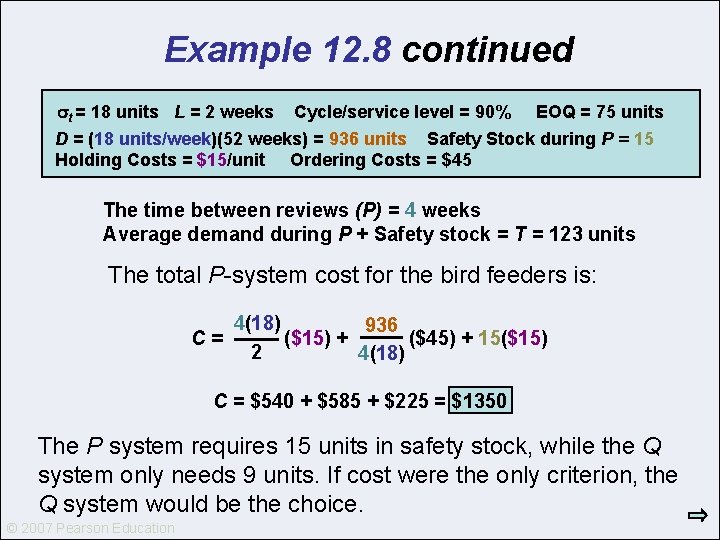
Example 12. 8 continued t = 18 units L = 2 weeks Cycle/service level = 90% EOQ = 75 units D = (18 units/week)(52 weeks) = 936 units Safety Stock during P = 15 Holding Costs = $15/unit Ordering Costs = $45 The time between reviews (P) = 4 weeks Average demand during P + Safety stock = T = 123 units The total P-system cost for the bird feeders is: 4(18) 936 C = ($15) + ($45) + 15($15) 2 4(18) C = $540 + $585 + $225 = $1350 The P system requires 15 units in safety stock, while the Q system only needs 9 units. If cost were the only criterion, the QPearson system would be the choice. © 2007 Education © 2007 Pearson Education

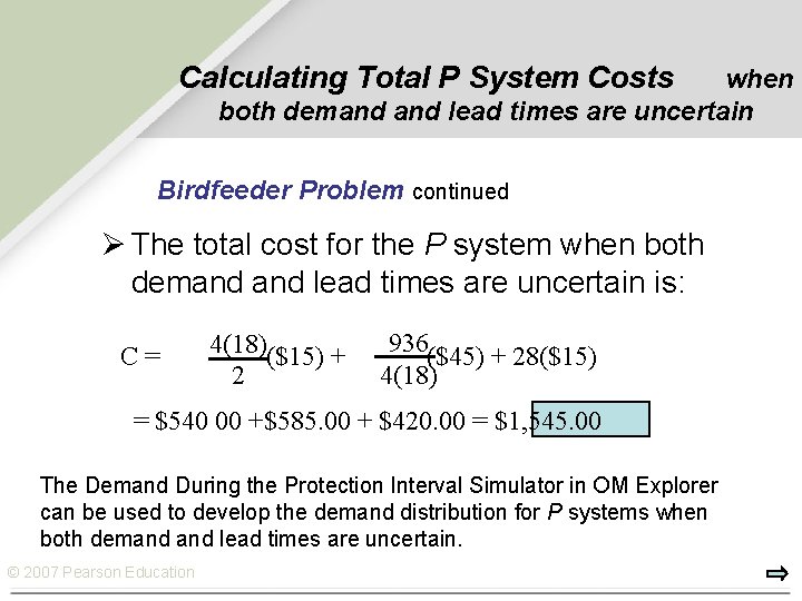
Calculating Total P System Costs when both demand lead times are uncertain Birdfeeder Problem continued Ø The total cost for the P system when both demand lead times are uncertain is: C= 4(18)($15) + 2 936($45) + 28($15) 4(18) = $540 00 +$585. 00 + $420. 00 = $1, 545. 00 The Demand During the Protection Interval Simulator in OM Explorer can be used to develop the demand distribution for P systems when both demand lead times are uncertain. © 2007 Pearson Education

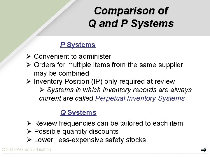
Comparison of Q and P Systems Ø Convenient to administer Ø Orders for multiple items from the same supplier may be combined Ø Inventory Position (IP) only required at review Ø Systems in which inventory records are always current are called Perpetual Inventory Systems Q Systems Ø Review frequencies can be tailored to each item Ø Possible quantity discounts Ø Lower, less-expensive safety stocks © 2007 Pearson Education

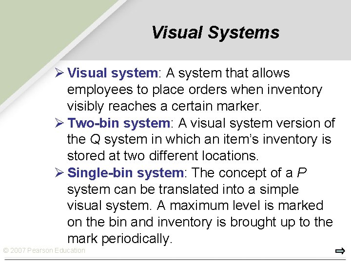
Visual Systems Ø Visual system: A system that allows employees to place orders when inventory visibly reaches a certain marker. Ø Two-bin system: A visual system version of the Q system in which an item’s inventory is stored at two different locations. Ø Single-bin system: The concept of a P system can be translated into a simple visual system. A maximum level is marked on the bin and inventory is brought up to the mark periodically. © 2007 Pearson Education

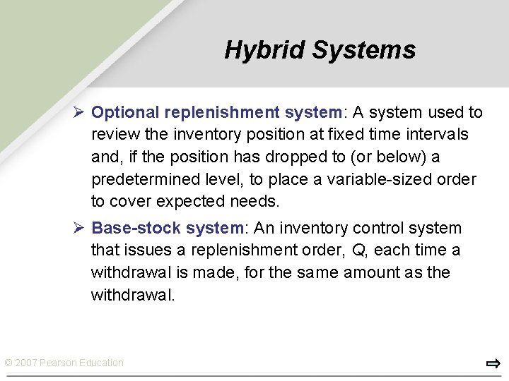
Hybrid Systems Ø Optional replenishment system: A system used to review the inventory position at fixed time intervals and, if the position has dropped to (or below) a predetermined level, to place a variable-sized order to cover expected needs. Ø Base-stock system: An inventory control system that issues a replenishment order, Q, each time a withdrawal is made, for the same amount as the withdrawal. © 2007 Pearson Education

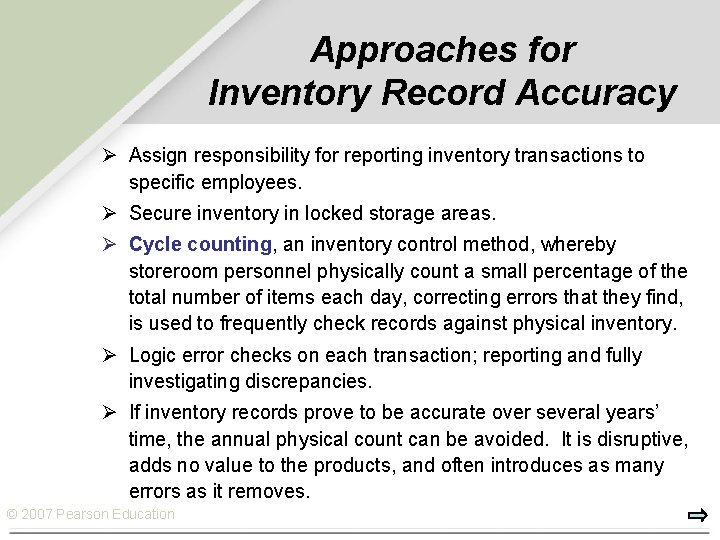
Approaches for Inventory Record Accuracy Ø Assign responsibility for reporting inventory transactions to specific employees. Ø Secure inventory in locked storage areas. Ø Cycle counting, an inventory control method, whereby storeroom personnel physically count a small percentage of the total number of items each day, correcting errors that they find, is used to frequently check records against physical inventory. Ø Logic error checks on each transaction; reporting and fully investigating discrepancies. Ø If inventory records prove to be accurate over several years’ time, the annual physical count can be avoided. It is disruptive, adds no value to the products, and often introduces as many errors as it removes. © 2007 Pearson Education

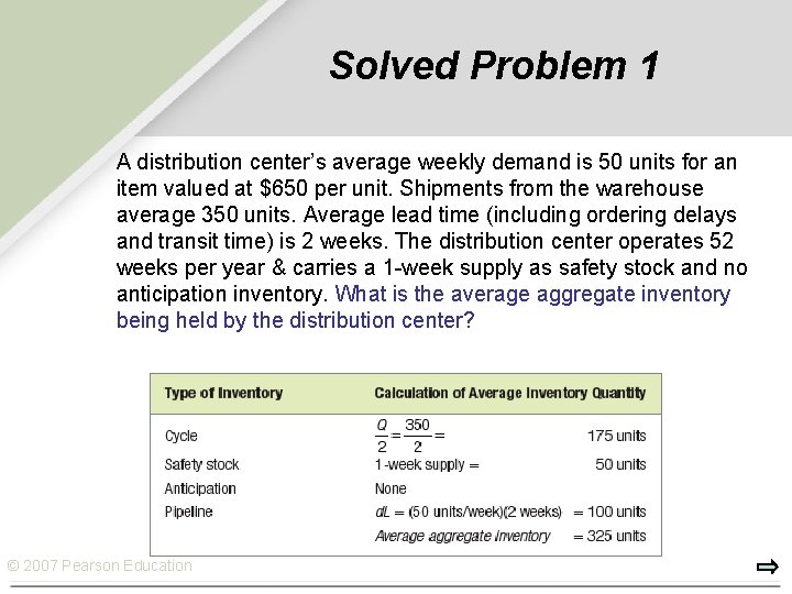
Solved Problem 1 A distribution center’s average weekly demand is 50 units for an item valued at $650 per unit. Shipments from the warehouse average 350 units. Average lead time (including ordering delays and transit time) is 2 weeks. The distribution center operates 52 weeks per year & carries a 1 -week supply as safety stock and no anticipation inventory. What is the average aggregate inventory being held by the distribution center? © 2007 Pearson Education

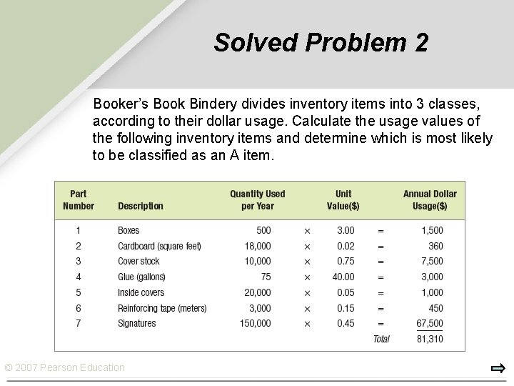
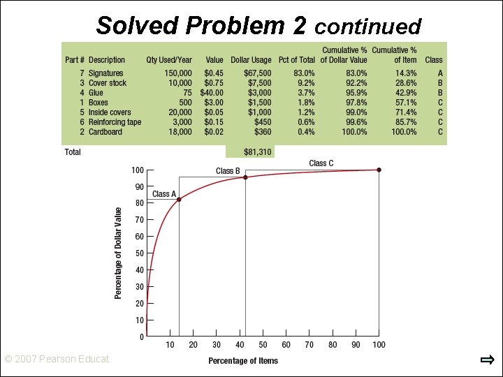
Solved Problem 2 Booker’s Book Bindery divides inventory items into 3 classes, according to their dollar usage. Calculate the usage values of the following inventory items and determine which is most likely to be classified as an A item. © 2007 Pearson Education

Solved Problem 2 continued © 2007 Pearson Education

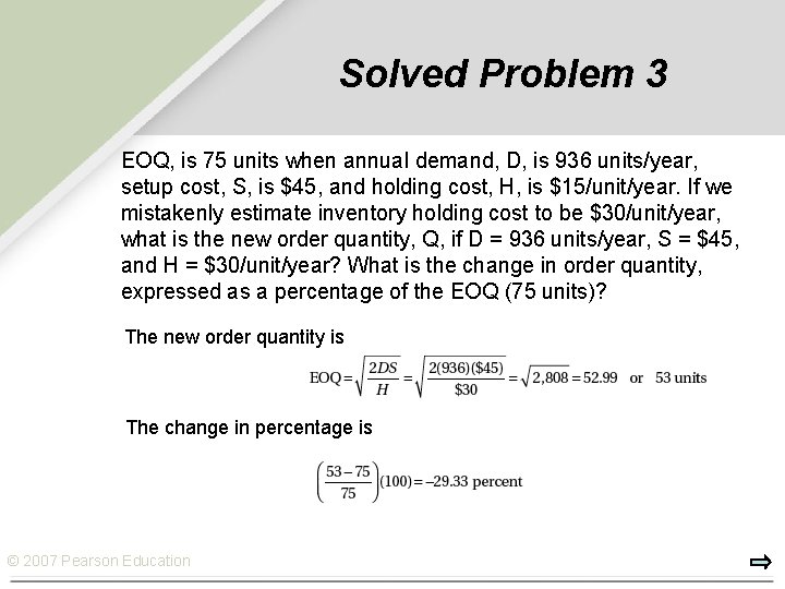
Solved Problem 3 EOQ, is 75 units when annual demand, D, is 936 units/year, setup cost, S, is $45, and holding cost, H, is $15/unit/year. If we mistakenly estimate inventory holding cost to be $30/unit/year, what is the new order quantity, Q, if D = 936 units/year, S = $45, and H = $30/unit/year? What is the change in order quantity, expressed as a percentage of the EOQ (75 units)? The new order quantity is The change in percentage is © 2007 Pearson Education

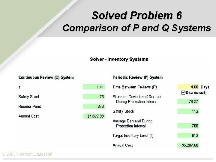
Solved Problem 6 Comparison of P and Q Systems © 2007 Pearson Education