Statistical Downscaling Hans von Storch Institute for Coastal

Statistical Downscaling Hans von Storch Institute for Coastal Research GKSS Research Centre Geesthacht, Germany 18. 10. 2004 Central Weather Bureau, Taipei, Taiwan

"Downscaling" is based on the view that regional climate is conditioned by climate on larger, for instance continental or even planetary, scales. Information is cascaded "down" from larger to smaller scales. The regional climate is the result of interplay of the overall atmospheric, or oceanic, circulation and of regional specifics, such as topography, land-sea distribution and land-use. As such, empirical/statistical downscaling seeks to derive the local scale information from the larger scale through inference from the cross-scale relationships, using a function F such that: local climate response = F (external, large scale forcing) Institut für Küstenforschung Concept of Empirical Downscaling If. K

Institut für Küstenforschung Concept of Empirical Downscaling If. K

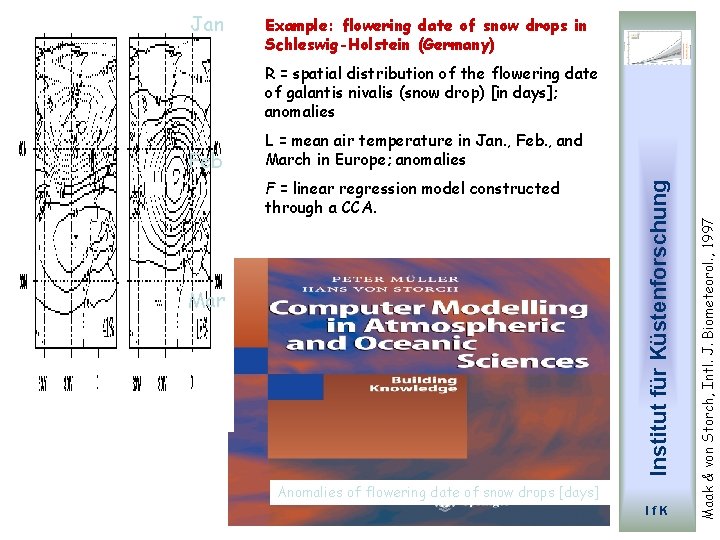
Jan Example: flowering date of snow drops in Schleswig-Holstein (Germany) R = spatial distribution of the flowering date of galantis nivalis (snow drop) [in days]; anomalies Mar Anomalies of flowering date of snow drops [days] If. K Maak & von Storch, Intl. J. Biometeorol. , 1997 F = linear regression model constructed through a CCA. Institut für Küstenforschung Feb L = mean air temperature in Jan. , Feb. , and March in Europe; anomalies

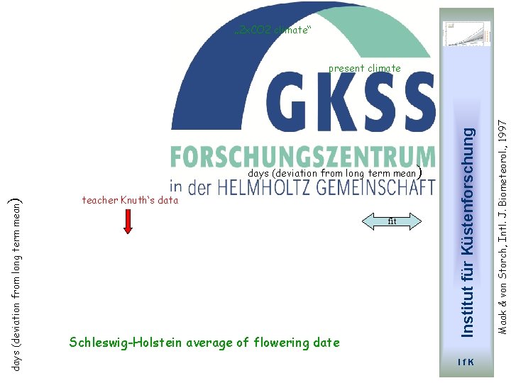
„ 2 x. CO 2 climate“ teacher Knuth‘s data fit Schleswig-Holstein average of flowering date ) If. K Maak & von Storch, Intl. J. Biometeorol. , 1997 days (deviation from long term mean ) days (deviation from long term mean Institut für Küstenforschung present climate

(1) The predictors are variables of relevance and are realistically modeled by the AOGCM. (2) The transfer function is valid also under altered climatic conditions. This is an assumption that in principle can not be proven in advance. The observational record should cover a wide range of variations in the past; ideally, all expected future realizations of the predictors should be contained in the observational record. (3) The predictors employed fully represent the climate change signal. Institut für Küstenforschung When using downscaling for assessing regional climate change, three implicit assumptions are made: If. K

Behind the concept stands the view that there is a "true“ function F, with a unique value F(L) for any large scale forcing L. Thus F may be thought of a “surface”, with L representing generalized coordinates – thus as a “terrain” F and geographical coordinates L. For the following, see: von Storch. , H. , 1999: Representation of conditional random distributions as a problem of "spatial" interpolation. In. J. Gòmez-Hernàndez, A. Soares and R. Froidevaux (Eds. ): geo. ENV II - Geostatistics for Environmental Applications. Kluwer Adacemic Publishers, Dordrecht, Boston, London, ISBN 0 -7923 -5783 -3, 13 -23 Institut für Küstenforschung local climate response = F (external, large scale forcing) If. K

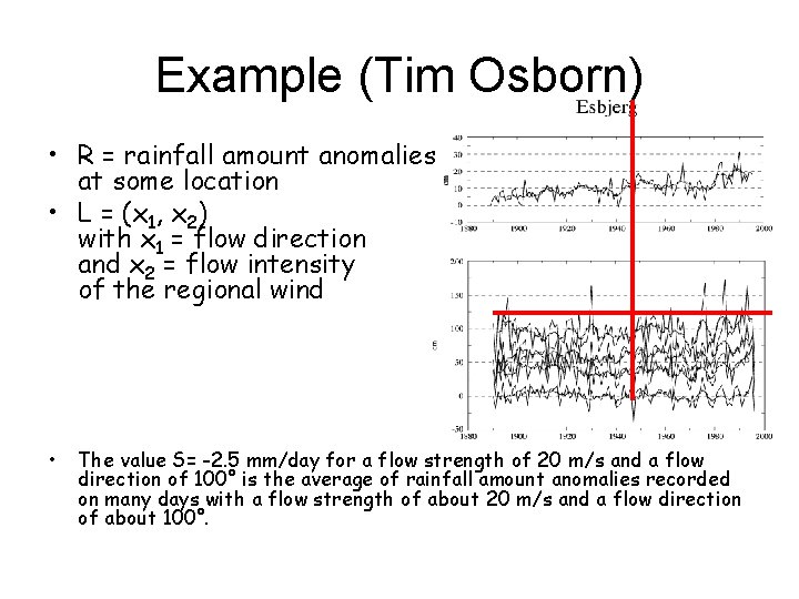
Example (Tim Osborn) • R = rainfall amount anomalies at some location • L = (x 1, x 2) with x 1 = flow direction and x 2 = flow intensity of the regional wind • The value S= -2. 5 mm/day for a flow strength of 20 m/s and a flow direction of 100° is the average of rainfall amount anomalies recorded on many days with a flow strength of about 20 m/s and a flow direction of about 100°.

The results of the interpolation is an approximate or estimated surface FE, which differs to some extend from the true surface F. The purpose of the spatial interpolation is the determination of the continuous surface F and not the reproduction of known points Fk. Institut für Küstenforschung Of course, the surface F is unknown. It needs to be determined by interpolating or approximating a number of point observations Fk at some “locations” Lk. This can be done by a number of different “spatial” interpolation methods. If. K

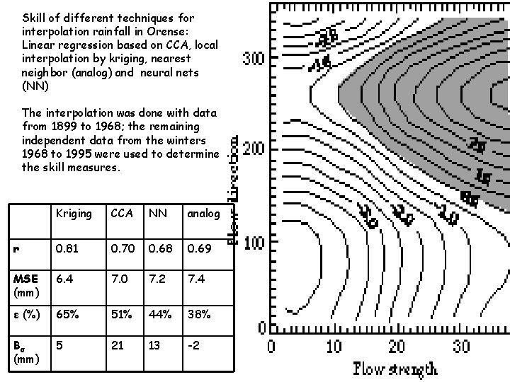
The success of FE, as an estimator of F may be determined by comparing the estimates FE(Lk) with the true F(Lk) at a number of additional data points. "Additional" means that the data F(Lk) have not used for determining FE. Conventional measures of success are • the bias, in the mean or in the standard deviation, i. e. , B =<FE(L)> – <F(L)>, Bσ = σE - σ , where the brackets <> represent the averaging operation over all considered data points L. σE and σ are standard deviations of FE(L) and of F(L). • the mean square root difference, i. e. , the squared correlation, i. e. , MSE =<FE(L) × F(L)>2 / <FE(L)2><F(L)2> • the represented variance ε = 1 – MSE / <F(L)2> Institut für Küstenforschung Skill of approximation If. K

• When we think of the “surface” no longer as a terrain but as the surface of the ocean, there is no longer a well defined height but a variable surface which elevation may be described in probabilistic terms. • Precipitation can not completely be understood as a function of the variables L (i. e. , as a function of flow direction and strength), but must in part be understood as being random. • The concept of "downscaling" does not imply that the regional climate would be determined by the large-scale state; for similar large-scale states, the associated regional states may vary substantially. Instead, the state is constrained or conditioned. • The regional climate is a random process conditioned upon a driving large-scale climate regime. That is, precipitation may be modeled as a random variable R conditioned upon flow direction and strength. The surface F is the conditional expectation E of R F(L) = E(R|L). Institut für Küstenforschung Random character of the problem If. K

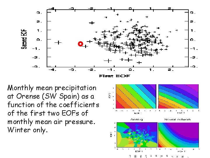
Monthly mean precipitation at Orense (SW Spain) as a function of the coefficients of the first two EOFs of monthly mean air pressure. Winter only.

Skill of different techniques for interpolation rainfall in Orense: Linear regression based on CCA, local interpolation by kriging, nearest neighbor (analog) and neural nets (NN) The interpolation was done with data from 1899 to 1968; the remaining independent data from the winters 1968 to 1995 were used to determine the skill measures. Kriging CCA NN analog r 0. 81 0. 70 0. 68 0. 69 MSE (mm) 6. 4 7. 0 7. 2 7. 4 ε (%) 65% 51% 44% 38% Bσ (mm) 5 21 13 -2

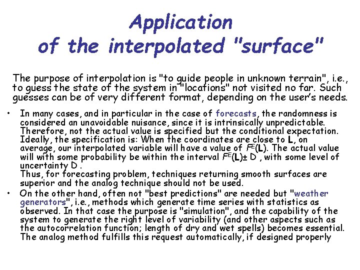
Application of the interpolated "surface" The purpose of interpolation is "to guide people in unknown terrain", i. e. , to guess the state of the system in "locations" not visited no far. Such guesses can be of very different format, depending on the user’s needs. • • In many cases, and in particular in the case of forecasts, the randomness is considered an unavoidable nuisance, since it is intrinsically unpredictable. Therefore, not the actual value is specified but the conditional expectation. Ideally, the specification is: When the coordinates are close to L, on average, our interpolated variable will have a value of FE(L). The actual value will with some probability be within the interval FE(L)± D , with some level of uncertainty D. Thus, forecasting problem, techniques returning smooth surfaces are superior and the analog technique should not be used. On the other hand, often not "best predictions" are needed but "weather generators", i. e. , methods which generate time series with statistics as observed. In that case the purpose is "simulation", and the capability of the system to generate the right level of variability (and other aspects such as the autocorrelation function; length of dry and wet spells) becomes essential. The analog method fulfills this request automatically, if designed properly

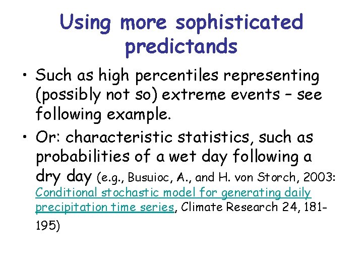
Using more sophisticated predictands • Such as high percentiles representing (possibly not so) extreme events – see following example. • Or: characteristic statistics, such as probabilities of a wet day following a dry day (e. g. , Busuioc, A. , and H. von Storch, 2003: Conditional stochastic model for generating daily precipitation time series, Climate Research 24, 181195)

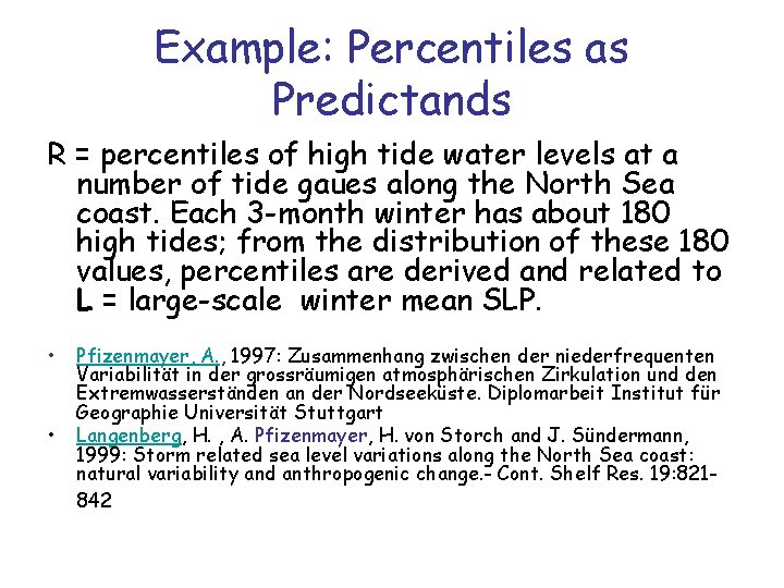
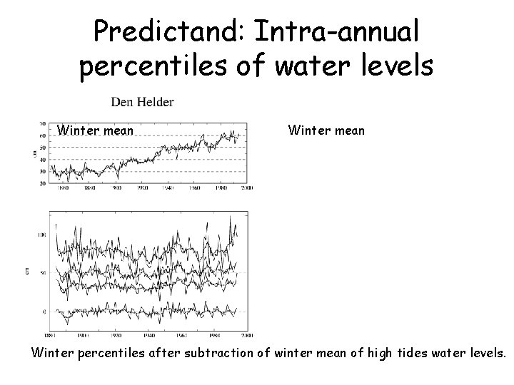
Example: Percentiles as Predictands R = percentiles of high tide water levels at a number of tide gaues along the North Sea coast. Each 3 -month winter has about 180 high tides; from the distribution of these 180 values, percentiles are derived and related to L = large-scale winter mean SLP. • • Pfizenmayer, A. , 1997: Zusammenhang zwischen der niederfrequenten Variabilität in der grossräumigen atmosphärischen Zirkulation und den Extremwasserständen an der Nordseeküste. Diplomarbeit Institut für Geographie Universität Stuttgart Langenberg, H. , A. Pfizenmayer, H. von Storch and J. Sündermann, 1999: Storm related sea level variations along the North Sea coast: natural variability and anthropogenic change. - Cont. Shelf Res. 19: 821842

Predictand: Intra-annual percentiles of water levels Winter mean Winter percentiles after subtraction of winter mean of high tides water levels.

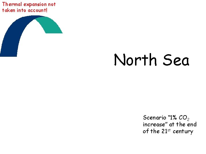
Thermal expansion not taken into account! North Sea Scenario “ 1% CO 2 increase” at the end of the 21 st century

End of examples Summary of range of methods 18. 10. 2004 Central Weather Bureau, Taipei, Taiwan

A diverse range of downscaling techniques methods has been developed, but in principle fall into three categories: (a) Weather generators, which are random number generators of realistically looking sequences conditioned upon the large-scale state. (b) Transfer functions, where a direct quantitative relationship is derived through, for example, regression. (c) Weather typing schemes based on the more traditional synoptic climatology concept (including analogs and phase space partitioning) and which relate a particular atmospheric state to a set of local climate variables. von Storch, H. , B. Hewitson and L. Mearns, 2000: Review of Empirical Downscaling Techniques. T. Iversen and B. A. K. Høiskar (Eds. ): Regional climate development under global warming. General Technical Report No. 4. Conf. Proceedings Reg. Clim Spring Meeting Jevnaker, Torbjørnrud, Norway, 8. - 9. May 2000, p. 29 -46

Weather generators are statistical models of observed sequences of weather variables. They can also be regarded as complex random number generators, the outputs of which resemble daily weather data at a particular location. There are two fundamental types of daily weather generators, based on the approach to modeling daily precipitation occurrence: the Markov chain approach and the spell-length approach. • In the Markov chain approach, a random process is constructed which determines a day at a station as rainy or dry, conditional upon the state of the previous day, following given probabilities. If a day is determined as rainy then the amount is drawn from a probability distribution. • In the spell length approach, the time between two rain days is modelled. For statistical downscaling the parameters of the weather generator are conditioned upon a large-scale state, or relationships can be developed between large-scale parameters sets of the weather generators and local scale parameters. See also: Giorgi, F. , B. Hewitson, J. Christensen, M. Hulme, H. von Storch, P. Whetton, R. Jones, L. Mearns and C. Fu, 2001: Regional climate information - evaluation and projections. In J. T. Houghton et al (eds. ): Climate Change 2001. The Scientific Basis, Cambridge University Press, 583 -638

Transfer functions - I The more common approaches found in the literature are regression-like techniques or piecewise interpolations using a linear or nonlinear formulation. The simplest approach is to build multiple regression models relating free atmosphere grid point values to surface variables. Canonical Correlation Analysis has found wide application. A variant of CCA is redundancy analysis, which is theoretically attractive as it maximizes the predictands variance; however, in practical terms it seems similar to CCA. Also Singular Value Decomposition has been used, which is another variant of CCA. Most applications have dealt with precipitation; another example has successfully specified local pressure tendencies, as a proxy for local storminess, from largescale monthly mean air pressure fields. Oceanic climate and climate impact variables have also been dealt with: salinity in the German Bight; and salinity and oxygen in the Baltic; sea level; and a number of ecological variables such as abundance of species. In addition statistics of extreme events, expressed as percentiles within a month or season, have been modeled: storm surge levels and ocean wave heights.

Transfer functions - II An alternative to linear regression is to use piecewise linear or nonlinear interpolation; geostatistics offers elegant "kriging" tools to this end. Another approach is to use cubic splines for specifying precipitation. Another non-linear approach is based on artificial neural networks (ANN), which are generally more powerful than other techniques, although the interpretation of the dynamical character of the relationships is less easy.

Weather typing • The synoptic downscaling approach empirically defines weather classes related to local and regional climate variations. These weather classes may be defined synoptically or fitted specifically for downscaling purposes by constructing indices of airflow. The mean, or frequency, distributions of local or regional climate are then derived by weighting the local climate states with the relative frequencies of the weather classes. Climate change is then estimated by determining the change of the frequency of weather classes. • In the "statistical/dynamical" approach, meso-scale atmospheric models are utilized for simulating a series of typical weather states. The advantage over the former technique is that in this way spatially distributed local climates are specified. • The applicability of the analog method was demonstrated mostly for the specification of daily precipitation. • Conceptually similar, but mathematically more demanding are techniques which partition the large-scale state phase space, for instance with Classification Tree Analysis, and use a randomized design for picking regional distributions. • Both analog and CART approaches return the right level of variance and correct spatial correlation structures.

Summary • Empirical downscaling methods have matured in the past years. • They are used for estimating a wide range of variables, both meteorological variables as well as statistics of not only meteorological but also oceanographic and ecological variables. • In some cases, dynamical downscaling does a better job, but many variables (e. g. ecological) can not dynamically modeled or are on spatial scales below the resolution of any RCM. • Thus, empirical downscaling is a method which will remain to play an important role for assessing ongoing change and projecting possibel future changes.

Downloads … • The ppt-file of this talk can be downloaded from http: //w 3 g. gkss. de/staff/storch/PPT/statistics. 041018. taipeh. ppt • Most of the literature given can be downloaded from http: //w 3 g. gkss. de/staff/storch/pub. htm http: //w 3 g. gkss. de/staff/storch/recent. htm http: //w 3 g. gkss. de/staff/storch/lit. htm

Advertisement Why do we think we build new knowledge by using complex models? Institut für Küstenforschung New book – If. K

Summary • Empirical downscaling methods have matured in the past years. • They are used for estimating a wide range of variables, both meteorological variables as well as statistics of not only meteorological but also oceanographic and ecological variables. • In some cases, dynamical downscaling does a better job, but many variables (e. g. ecological) can not dynamically modeled or are on spatial scales below the resolution of any RCM. • Thus, empirical downscaling is a method which will remain to play an important role for assessing ongoing change and projecting possibel future changes.

Downloads … • The ppt-file of this talk can be downloaded from http: //w 3 g. gkss. de/staff/storch/PPT/statistics/041018. taipeh. ppt • Most of the literature given can be downloaded from http: //w 3 g. gkss. de/staff/storch/pub. htm http: //w 3 g. gkss. de/staff/storch/recent. htm http: //w 3 g. gkss. de/staff/storch/lit. htm