Spatial Autocorrelation and Uncertainty Associated With Remotely Sensed

Spatial Autocorrelation and Uncertainty Associated With Remotely Sensed Data Daniel A. Griffith Ashbel Smith Professor of Geospatial Information Sciences & Yongwan Chun 1

Big Data, Statistics, and Environmental Sciences Results can be extended to billions+ of pixels An extension of spatial statistics to remote sensing work: Chen, X-L. ; H-M. Zhao; P-X Li; Z-Y Yin. Remote sensing image-based analysis of the relationship between urban heat island use/cover changes, Remote Sensing of Environment, 2006, 104, 133 -146. Ø Uses aspatial regression, and has 447 citations Relevant to spectral indices analysis The work most closely relates to Finley’s afternoon presentation: presentation Computational considerations for applying nearest neighbor Gaussian processes to large spatial data sets

ABSTRACT Ø Virtually all remotely sensed data contain spatial autocorrelation, which impacts upon their statistical features of uncertainty through variance inflation, and the compounding of duplicate information. Ø Estimating the nature and degree of this spatial autocorrelation, which usually is positive and very strong, has been hindered by computational intensity associated with the massive number of pixels in realistic sized remotely sensed images. Ø Recent advances in spatial statistical estimation theory support the extraction of information and the distilling of knowledge from remotely sensed images in a way that accounts for latent spatial autocorrelation. Ø This paper summarizes an effective methodological approach to achieve this end.

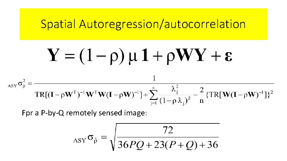
Spatial Autoregression/autocorrelation Fpr a P-by-Q remotely sensed image:

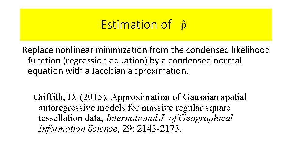
Estimation of xxx Replace nonlinear minimization from the condensed likelihood function (regression equation) by a condensed normal equation with a Jacobian approximation: Griffith, D. (2015). Approximation of Gaussian spatial autoregressive models for massive regular square tessellation data, International J. of Geographical Information Science, 29: 2143 -2173.

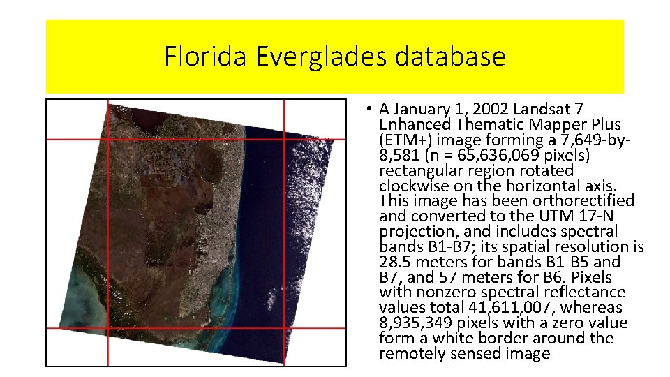
Florida Everglades database • A January 1, 2002 Landsat 7 Enhanced Thematic Mapper Plus (ETM+) image forming a 7, 649 -by 8, 581 (n = 65, 636, 069 pixels) rectangular region rotated clockwise on the horizontal axis. This image has been orthorectified and converted to the UTM 17 -N projection, and includes spectral bands B 1 -B 7; its spatial resolution is 28. 5 meters for bands B 1 -B 5 and B 7, and 57 meters for B 6. Pixels with nonzero spectral reflectance values total 41, 611, 007, whereas 8, 935, 349 pixels with a zero value form a white border around the remotely sensed image

Sampling Experiment Empirical Data Ø A 4800 -by-5200 (n = 24, 960, 000 pixels) rectangular region parallel to the horizontal axis was extracted for analysis purposes. Ø The sampling experiments use two spectral indices (both indices range from -1 to 1, and have a variance that conceptually can range from 0 to 1): v the normalized difference vegetation index [i. e. , NDVI = (B 4 -B 3)/(B 4+B 3)] v NDVI tends to be around 0. 95 (the Everglades image analyzed in this paper has a spatial autocorrelation of 0. 955), the common upper bound for many remotely sensed images v Large positive NDVI values indicate dense vegetation land cover, whereas large negative values indicate deep water v the normalized burn ratio [i. e. , NBR = (B 4 -B 7)/(B 4+B 7)]. v NBR tends to be around 0. 85 (the Everglades image analyzed in this paper has a spatial autocorrelation of 0. 874), the common lower bound for many remotely sensed images v Large positive NBR values indicate high severity burn, whereas large negative values indicate high post-fire regrowth.

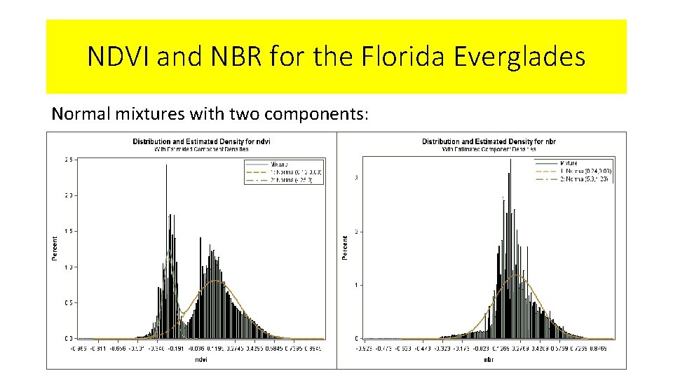
NDVI and NBR for the Florida Everglades Normal mixtures with two components:

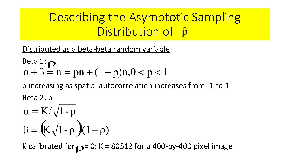
Describing the Asymptotic Sampling Distribution of xxx Distributed as a beta-beta random variable Beta 1: p increasing as spatial autocorrelation increases from -1 to 1 Beta 2: p K calibrated for = 0: K = 80512 for a 400 -by-400 pixel image

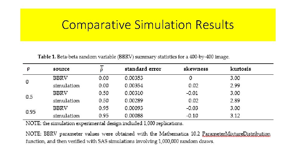
Comparative Simulation Results

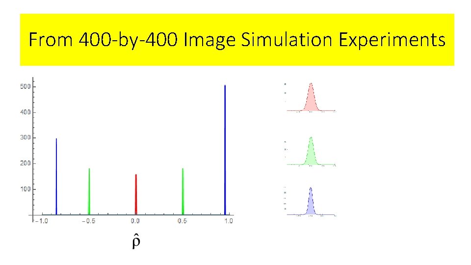
From 400 -by-400 Image Simulation Experiments

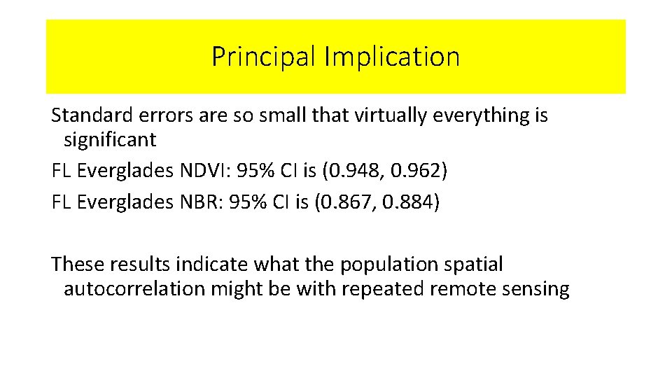
Principal Implication Standard errors are so small that virtually everything is significant FL Everglades NDVI: 95% CI is (0. 948, 0. 962) FL Everglades NBR: 95% CI is (0. 867, 0. 884) These results indicate what the population spatial autocorrelation might be with repeated remote sensing

Relevant Questions for Spatial Analysts What happens if I select an image in a different location? What happens if I select an image that is slightly shifted? What happens if I randomly sample my geographic landscape? What happens if I increase the scale of my geographic landscape?

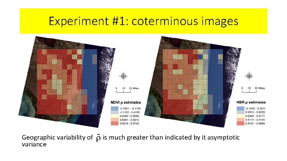
Experiment #1: coterminous images Geographic variability of variance is much greater than indicated by it asymptotic

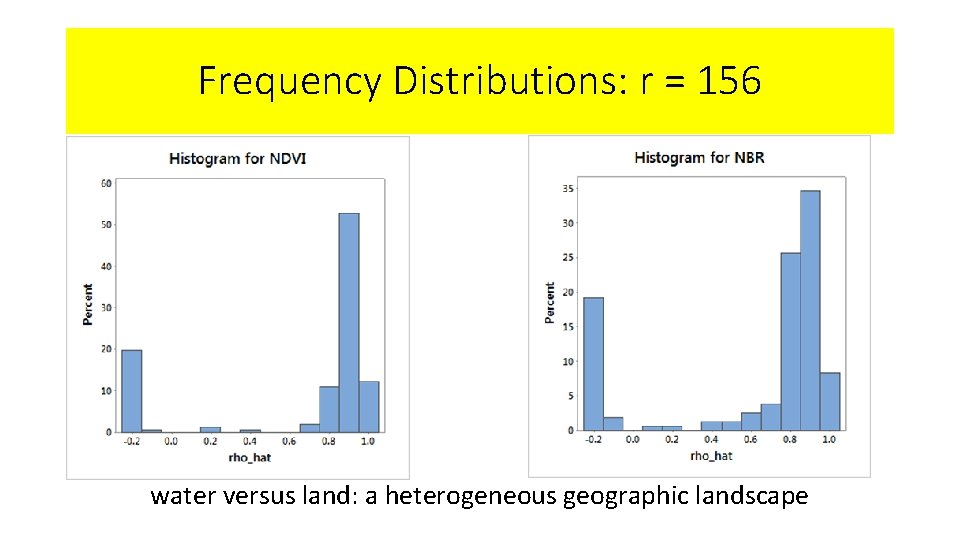
Frequency Distributions: r = 156 water versus land: a heterogeneous geographic landscape

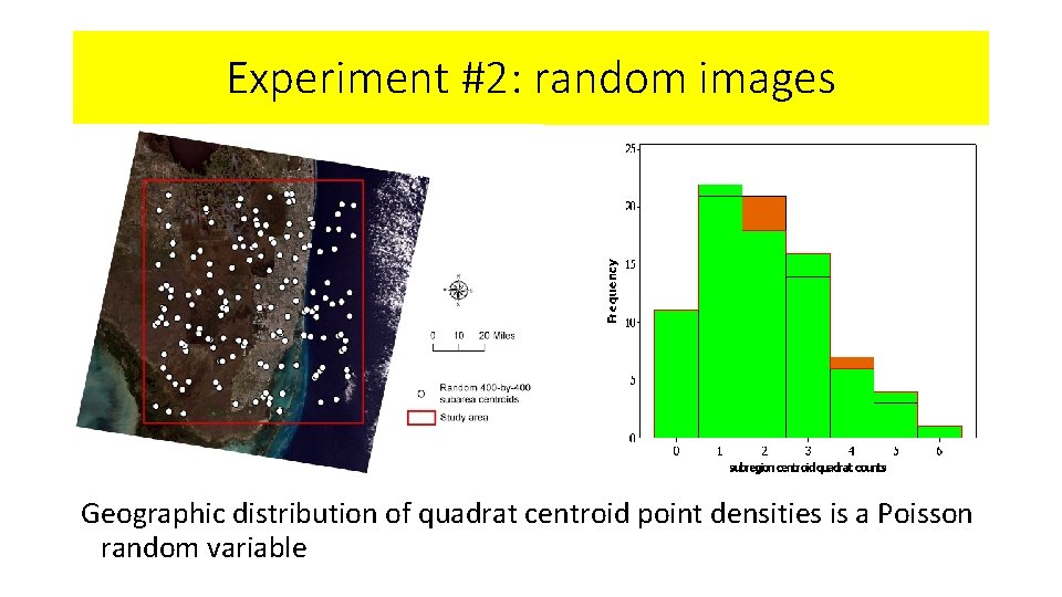
Experiment #2: random images Geographic distribution of quadrat centroid point densities is a Poisson random variable

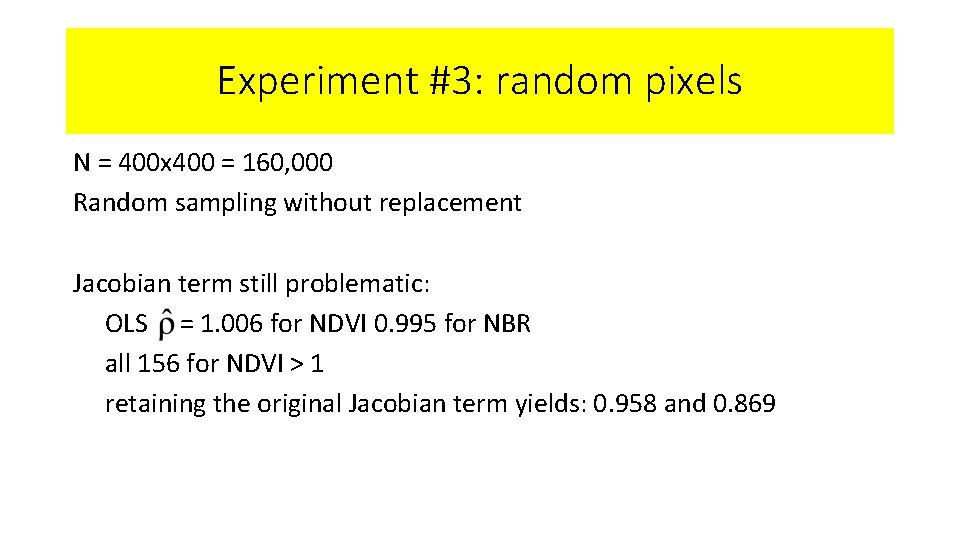
Experiment #3: random pixels N = 400 x 400 = 160, 000 Random sampling without replacement Jacobian term still problematic: OLS = 1. 006 for NDVI 0. 995 for NBR all 156 for NDVI > 1 retaining the original Jacobian term yields: 0. 958 and 0. 869

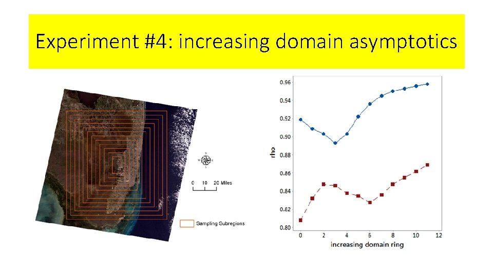
Experiment #4: increasing domain asymptotics

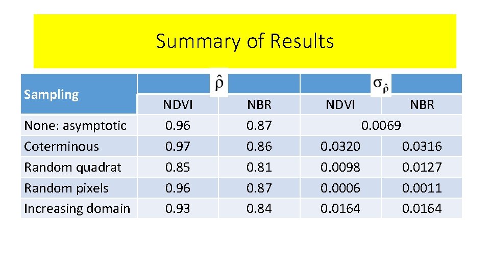
Summary of Results Sampling None: asymptotic Coterminous Random quadrat Random pixels Increasing domain NDVI 0. 96 0. 97 0. 85 0. 96 0. 93 NBR 0. 87 0. 86 0. 81 0. 87 0. 84 NDVI NBR 0. 0069 0. 0320 0. 0098 0. 0006 0. 0164 0. 0316 0. 0127 0. 0011 0. 0164

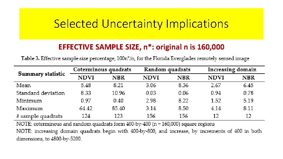
Selected Uncertainty Implications EFFECTIVE SAMPLE SIZE, n*: original n is 160, 000

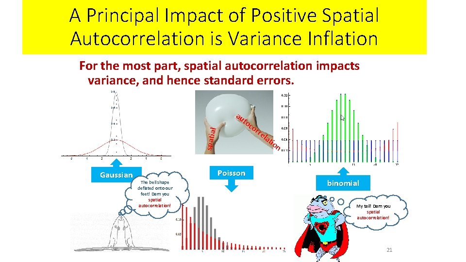
A Principal Impact of Positive Spatial Autocorrelation is Variance Inflation For the most part, spatial autocorrelation impacts variance, and hence standard errors. au spatia l to Gaussian Poisson The bell shape deflated onto our feet! Darn you spatial autocorrelation! co rre lat ion binomial My tail! Darn you spatial autocorrelation! 21

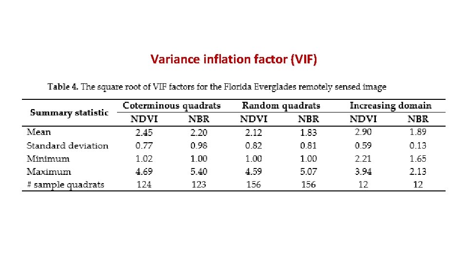
Variance inflation factor (VIF)

Some Concluding Comments Cressie, N. , A. Olsen, and D. Cook. 1996. Massive data sets: problems and possibilities, with application to environmental monitoring, in Massive Data Sets: Proceedings of a Workshop, edited by the Committee of Applied and Theoretical Statistics, pp. 115 -119. Washington, DC: National Academy Press. massively large georeferenced datasets challenge, and may ultimately cause the failure of, spatial statistical methodology initially designed for georeferenced datasets with n in the 100 s, which has been extended successfully and effectively to datasets with n in the 10, 000 s Statistical significance is one of these challenge areas. 3/7/2016: the American Statistical Association Board of Directors issued a statement on p-values and statistical significance.

Spatial Statistical Methodology Developments • Now supports estimation of spatial autoregressive model specifications for realistic remotely sensed images • Now supports simulation experiments for massively large georeferenced datasets that can include 10, 000 replications in order to exploit the Law of Large Numbers • Reveals that remotely sensed images have large VIFs • Quantifies that much information content in remotely sensed images is compounded duplicate information • Shifts some focus to negative spatial autocorrelation

25