Remotely sensed land cover heterogeneity MaoNing Tuanmu 5292012

Remotely sensed land cover heterogeneity Mao-Ning Tuanmu 5/29/2012

Outline Objectives & rationale Remotely sensed data Heterogeneity metrics Calculation approaches of heterogeneity metrics • Next steps • •

Spatial heterogeneity of land cover • Species distributions and biodiversity patterns • Landscape metrics based on categorical land cover maps – Boundary delineation – Heterogeneity within a land cover type • Continuous measures of land surface characteristics from remote sensing

Objectives • To explore different approaches for quantifying land cover heterogeneity based on remotely sensed data • To generate remote sensing-based heterogeneity metrics at the global scale • To evaluate the usefulness of those metrics for explaining biodiversity patterns and monitoring their temporal dynamics

Remote Sensing Imagery • Landsat 5 TM and Landsat 7 ETM+ • Global Land Survey (GLS) surface reflectance – 7 bands, QA – Three epochs: 1990, 2005 – 7, 000~8, 000+ scenes for each epoch – 22 scenes covering the entire Oregon • Vegetation indices – NDVI

Remote Sensing-Based Metrics • First-order texture measures – Statistics calculated from image pixel values – Composition of pixel values – Average, SD, range, maximum, minimum and etc. of pixel values within a pixel neighborhood – Values of individual spectral bands – Linear or non-linear combinations of spectral bands

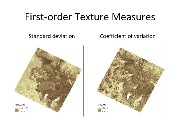
First-order Texture Measures Standard deviation Coefficient of variation

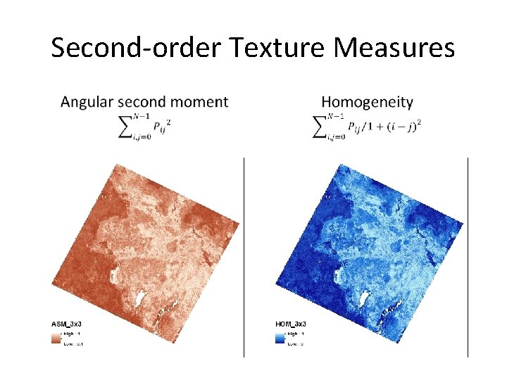
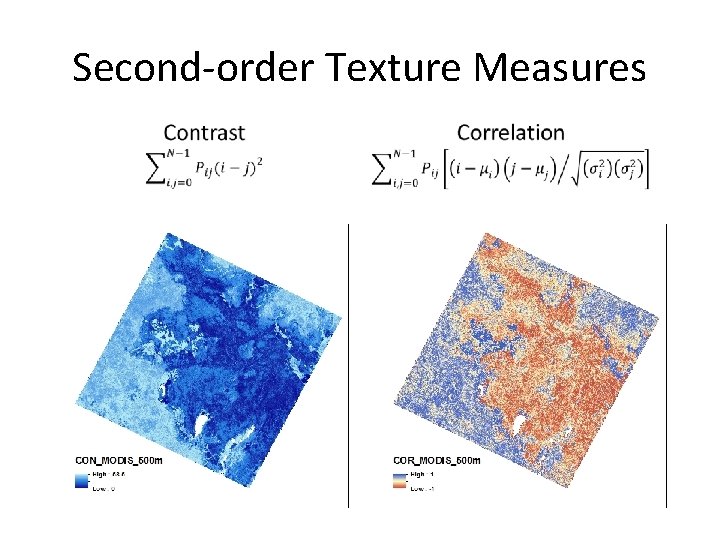
Remote Sensing-Based Metrics • Second-order texture measures – Statistics calculated based on values of pixel pairs – Information on the spatial relationship between two pixels – Spatial configuration (or arrangement) of pixel values – Metrics based on the Gray Level Co-occurrence Matrix (GLCM)

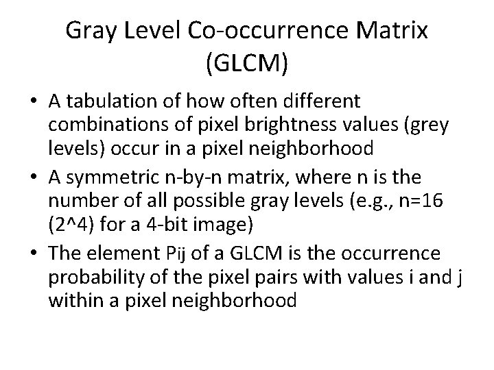
Gray Level Co-occurrence Matrix (GLCM) • A tabulation of how often different combinations of pixel brightness values (grey levels) occur in a pixel neighborhood • A symmetric n-by-n matrix, where n is the number of all possible gray levels (e. g. , n=16 (2^4) for a 4 -bit image) • The element Pij of a GLCM is the occurrence probability of the pixel pairs with values i and j within a pixel neighborhood

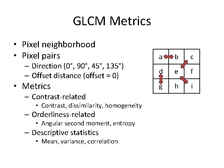
GLCM Metrics • Pixel neighborhood • Pixel pairs – Direction (0°, 90°, 45°, 135°) – Offset distance (offset = 0) • Metrics – Contrast-related • Contrast, dissimilarity, homogeneity – Orderliness-related • Angular second moment, entropy – Descriptive statistics • Mean, variance, correlation a b c d e f g h i

Second-order Texture Measures

Second-order Texture Measures

Moving Window vs. Fixed Grid • Moving window approach – Run a moving window across the entire image (study area) to calculate first- and second-order metrics for each pixel (e. g. , Landsat pixel of 30 m) – Aggregate metric values (e. g. , calculate mean and SD) for a larger regular grid (e. g. , MODIS 500 m grid) or specific area (e. g. , sampling plot) • Fixed grid approach – Directly calculate metrics based on the values of Landsat pixels within each MODIS pixel

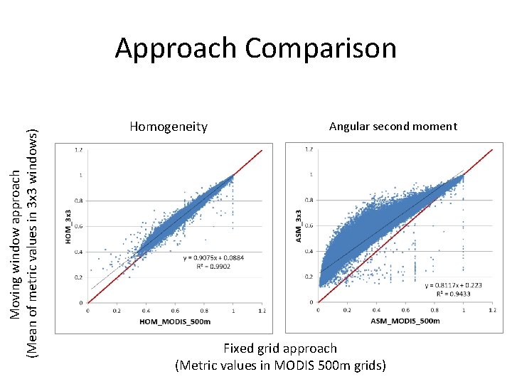
Moving window approach (Mean of metric values in 3 x 3 windows) Approach Comparison Homogeneity Angular second moment Fixed grid approach (Metric values in MODIS 500 m grids)

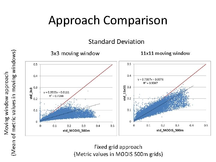
Approach Comparison Moving window approach (Mean of metric values in moving windows) Standard Deviation 3 x 3 moving window 11 x 11 moving window Fixed grid approach (Metric values in MODIS 500 m grids)

Moving Window vs. Fixed Grid • Moving window approach – Texture characteristics at different grains (3 x 3, 11 x 11…) – Computation-intensive • Fixed grid approach – Texture characteristics at the scale of the fixed grid – Easier to interpret – Much less computation-intensive (> 10 times faster)

Next Steps • Comparison between texture measures and landscape metrics from categorical land cover data (NLCD) – Fragstats – Only in the Windows system – Cannot handle the entire Landsat scene with the moving window approach

Next Steps • Metrics related to spatial autocorrelation – Measures of spatial autocorrelation (e. g. , Moran’s I) – Characteristics of variogram (e. g. , sill and range) • Seasonality effects – Cropland – Mosaicked images from NASA