Parametric and NonParametric analysis of complex diseases Lecture

Parametric and Non-Parametric analysis of complex diseases Lecture #6 Based on: Chapter 25 & 26 in Terwilliger and Ott’s Handbook of Human Genetic Linkage. . Prepared by Dan Geiger.

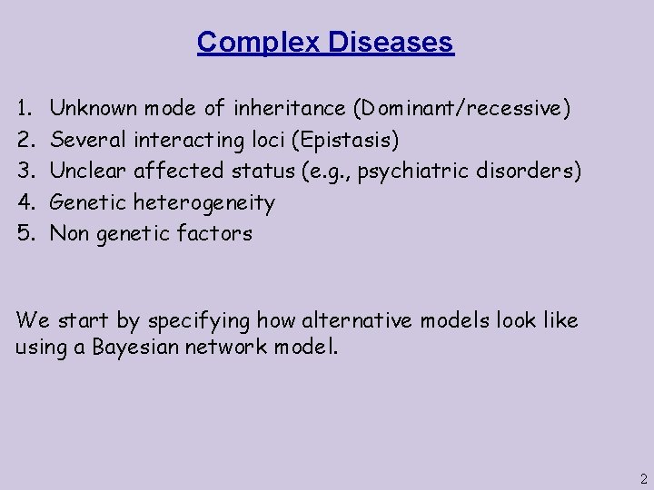
Complex Diseases 1. 2. 3. 4. 5. Unknown mode of inheritance (Dominant/recessive) Several interacting loci (Epistasis) Unclear affected status (e. g. , psychiatric disorders) Genetic heterogeneity Non genetic factors We start by specifying how alternative models look like using a Bayesian network model. 2

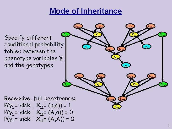
Mode of Inheritance L 11 m L 12 m L 11 f X 11 S 13 m Specify different conditional probability tables between the phenotype variables Yi and the genotypes y 1 L 12 f X 12 y 2 L 13 f L 13 m S 13 f X 13 y 3 L 21 m S 23 m Recessive, full penetrance: P(y 1 = sick | X 11= (a, a)) = 1 P(y 1 = sick | X 11= (A, a)) = 0 P(y 1 = sick | X 11= (A, A)) = 0 L 22 m L 21 f X 21 X 22 L 22 f S 23 f L 23 m X 23 3

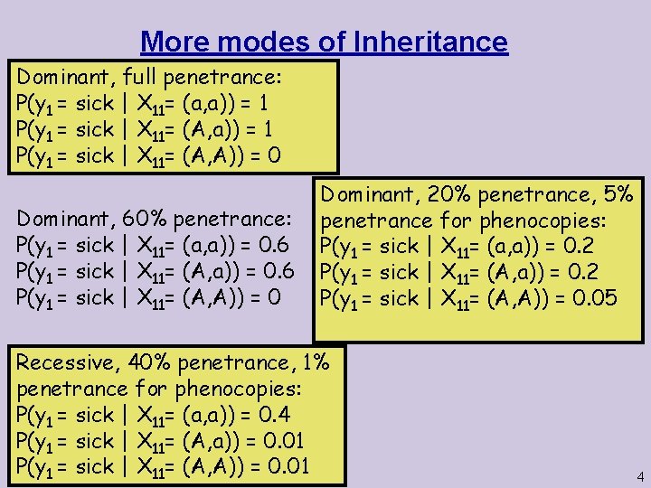
More modes of Inheritance Dominant, full penetrance: P(y 1 = sick | X 11= (a, a)) = 1 P(y 1 = sick | X 11= (A, A)) = 0 Dominant, 60% penetrance: P(y 1 = sick | X 11= (a, a)) = 0. 6 P(y 1 = sick | X 11= (A, A)) = 0 Dominant, 20% penetrance, 5% penetrance for phenocopies: P(y 1 = sick | X 11= (a, a)) = 0. 2 P(y 1 = sick | X 11= (A, A)) = 0. 05 Recessive, 40% penetrance, 1% penetrance for phenocopies: P(y 1 = sick | X 11= (a, a)) = 0. 4 P(y 1 = sick | X 11= (A, a)) = 0. 01 P(y 1 = sick | X 11= (A, A)) = 0. 01 4

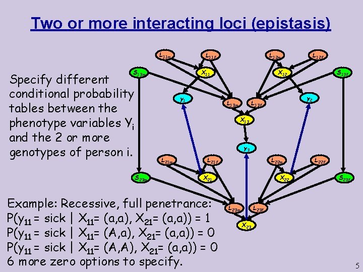
Two or more interacting loci (epistasis) L 11 m X 11 S 13 m Specify different conditional probability tables between the phenotype variables Yi and the 2 or more genotypes of person i. L 12 m L 11 f y 1 L 12 f X 12 y 2 L 13 f L 13 m S 13 f X 13 y 3 L 21 m S 23 m L 22 m L 21 f X 21 Example: Recessive, full penetrance: P(y 11 = sick | X 11= (a, a), X 21= (a, a)) = 1 P(y 11 = sick | X 11= (A, a), X 21= (a, a)) = 0 P(y 11 = sick | X 11= (A, A), X 21= (a, a)) = 0 6 more zero options to specify. X 22 L 22 f S 23 f L 23 m X 23 5

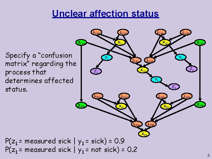
Unclear affection status L 11 m X 11 S 13 m Specify a “confusion matrix” regarding the process that determines affected status. L 12 m L 11 f Y 1 L 12 f X 12 S 13 f Y 2 L 13 f L 13 m Z 1 X 13 Z 1 Y 3 Z 1 L 21 m S 23 m L 22 m L 21 f X 21 X 22 S 23 f L 23 m P(z 1 = measured sick | y 1 = sick) = 0. 9 P(z 1 = measured sick | y 1 = not sick) = 0. 2 L 22 f X 23 6

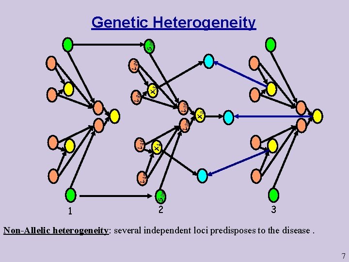
Xi 3 Xi 1 Si 3 m Li 1 f Li 3 m Li 3 f Xi 2 Li 2 m Li 2 f Si 3 f Genetic Heterogeneity 1 2 3 Non-Allelic heterogeneity: several independent loci predisposes to the disease. 7

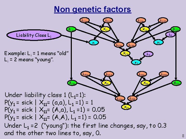
Non genetic factors L 11 m Liability Class L 12 m L 11 f X 11 S 13 m L 12 f X 12 S 13 f L 2 y 1 Example: Li = 1 means “old” Li = 2 means “young”. y 2 L 13 f L 13 m X 13 L 3 y 3 L 21 m S 23 m L 22 m L 21 f X 21 L 22 f X 22 Under liability class 1 (L 1=1): L L P(y 1 = sick | X 11= (a, a), L 1 =1) = 1 X P(y 1 = sick | X 11= (A, a), L 1 =1) = 0. 05 P(y 1 = sick | X 11= (A, A), L 1 =1) = 0. 05 Under L 1 =2 (“young”): the first line changes, say, to 0. 3 and the other two lines to, say, 0. S 23 f 23 m 23 8

Parametric versus Non-Parametric All analyses considered so far are “parametric” meaning that a mode of inheritance is assumed. In some cases, several options of modes of inheritance are assumed but still the analysis uses each option in turn. For complex diseases it is believed that “non-parametric” methods might work better. In our context, these are methods that do not take mode of inheritance into account. The idea is that computing linkage without assuming mode of inheritance is more robust to error in model specification. Clearly, if the model is correct, parametric methods perform better, but not so if the model is wrong as for complex traits. 9

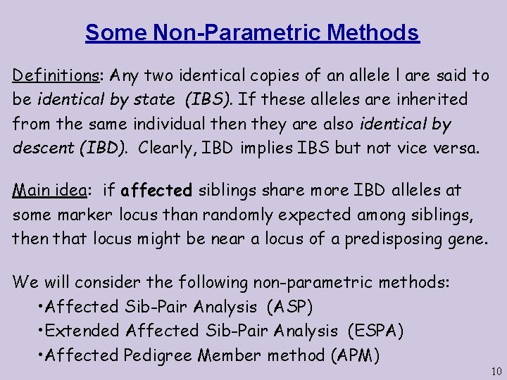
Some Non-Parametric Methods Definitions: Any two identical copies of an allele l are said to be identical by state (IBS). If these alleles are inherited from the same individual then they are also identical by descent (IBD). Clearly, IBD implies IBS but not vice versa. Main idea: if affected siblings share more IBD alleles at some marker locus than randomly expected among siblings, then that locus might be near a locus of a predisposing gene. We will consider the following non-parametric methods: • Affected Sib-Pair Analysis (ASP) • Extended Affected Sib-Pair Analysis (ESPA) • Affected Pedigree Member method (APM) 10

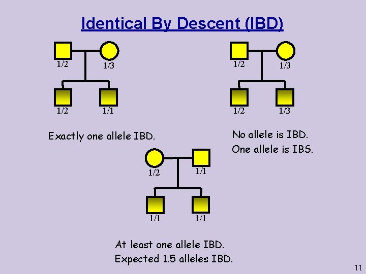
Identical By Descent (IBD) 1/2 1/3 1/2 1/1 1/2 1/3 No allele is IBD. One allele is IBS. Exactly one allele IBD. 1/2 1/1 1/1 At least one allele IBD. Expected 1. 5 alleles IBD. 11

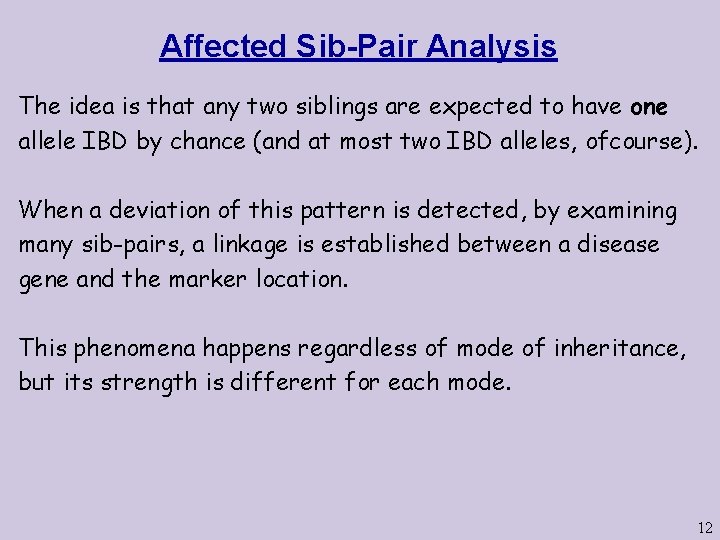
Affected Sib-Pair Analysis The idea is that any two siblings are expected to have one allele IBD by chance (and at most two IBD alleles, ofcourse). When a deviation of this pattern is detected, by examining many sib-pairs, a linkage is established between a disease gene and the marker location. This phenomena happens regardless of mode of inheritance, but its strength is different for each mode. 12

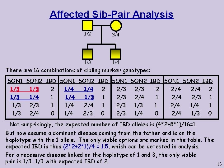
Affected Sib-Pair Analysis 1/2 3/4 1/3 There are 16 combinations of sibling marker genotypes: SON 1 SON 2 IBD 1/3 2 1/4 2 2/3 2 2/4 2 1/3 1/4 1/3 1 2/3 2/4 1 2/4 2/3 1 1/3 2/3 1 1/4 2/4 1 2/3 1 2/4 1 1/3 2/4 0 1/4 2/3 0 2/3 1/4 0 2/4 1/3 0 Not surprisingly, the expected number of IBD alleles is (4*2+8*1)/16=1. But now assume a dominant disease coming from the father and is on the haplotype with the 1 allele. The only viable options are marked in the table. The expected IBD is thus (2*2+2*1)/4 = 1. 5, which can be detected in analysis. For a recessive disease linked on the haplotype of 1 and 3, the only viable pair is 1/3, 1/3 with expected IBD of 2. 13

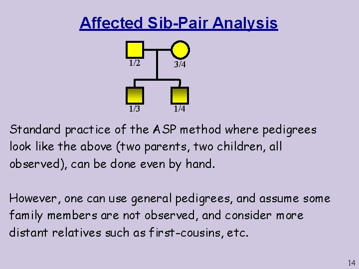
Affected Sib-Pair Analysis 1/2 3/4 1/3 1/4 Standard practice of the ASP method where pedigrees look like the above (two parents, two children, all observed), can be done even by hand. However, one can use general pedigrees, and assume some family members are not observed, and consider more distant relatives such as first-cousins, etc. 14

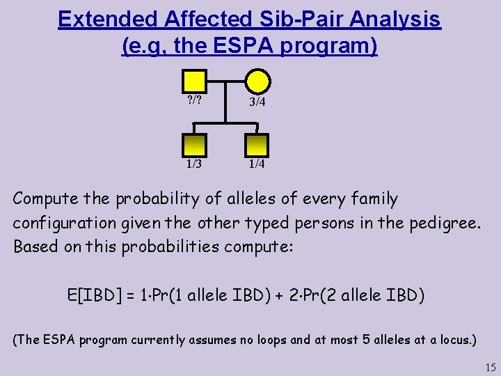
Extended Affected Sib-Pair Analysis (e. g, the ESPA program) ? /? 3/4 1/3 1/4 Compute the probability of alleles of every family configuration given the other typed persons in the pedigree. Based on this probabilities compute: E[IBD] = 1 Pr(1 allele IBD) + 2 Pr(2 allele IBD) (The ESPA program currently assumes no loops and at most 5 alleles at a locus. ) 15

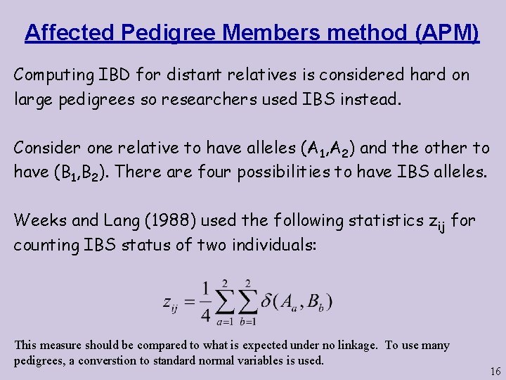
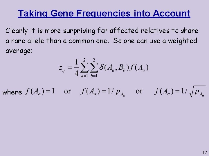
Affected Pedigree Members method (APM) Computing IBD for distant relatives is considered hard on large pedigrees so researchers used IBS instead. Consider one relative to have alleles (A 1, A 2) and the other to have (B 1, B 2). There are four possibilities to have IBS alleles. Weeks and Lang (1988) used the following statistics zij for counting IBS status of two individuals: This measure should be compared to what is expected under no linkage. To use many pedigrees, a converstion to standard normal variables is used. 16

Taking Gene Frequencies into Account Clearly it is more surprising for affected relatives to share a rare allele than a common one. So one can use a weighted average: where 17