10 Parametric Equations and Polar Coordinates Copyright Cengage

10 Parametric Equations and Polar Coordinates Copyright © Cengage Learning. All rights reserved.

10. 3 Polar Coordinates Copyright © Cengage Learning. All rights reserved.

Polar Coordinates A coordinate system represents a point in the plane by an ordered pair of numbers called coordinates. Usually we use Cartesian coordinates, which are directed distances from two perpendicular axes. Here we describe a coordinate system introduced by Newton, called the polar coordinate system, which is more convenient for many purposes. We choose a point in the plane that is called the pole (or origin) and is labeled O. Then we draw a ray (half-line) starting at O called the polar axis. 3

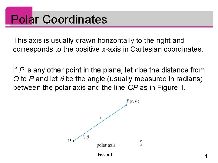
Polar Coordinates This axis is usually drawn horizontally to the right and corresponds to the positive x-axis in Cartesian coordinates. If P is any other point in the plane, let r be the distance from O to P and let be the angle (usually measured in radians) between the polar axis and the line OP as in Figure 1 4

Polar Coordinates Then the point P is represented by the ordered pair (r, ) and r, are called polar coordinates of P. We use the convention that an angle is positive if measured in the counterclockwise direction from the polar axis and negative in the clockwise direction. If P = O, then r = 0 and we agree that (0, ) represents the pole for any value of . 5

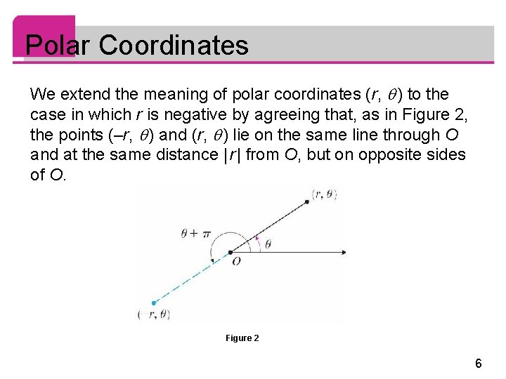
Polar Coordinates We extend the meaning of polar coordinates (r, ) to the case in which r is negative by agreeing that, as in Figure 2, the points (–r, ) and (r, ) lie on the same line through O and at the same distance | r | from O, but on opposite sides of O. Figure 2 6

Polar Coordinates If r 0, the point (r, ) lies in the same quadrant as ; if r 0, it lies in the quadrant on the opposite side of the pole. Notice that (–r, ) represents the same point as (r, + ). 7

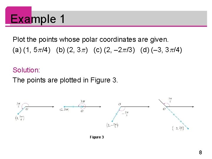
Example 1 Plot the points whose polar coordinates are given. (a) (1, 5 /4) (b) (2, 3 ) (c) (2, – 2 /3) (d) (– 3, 3 /4) Solution: The points are plotted in Figure 3 8

Example 1 – Solution cont’d In part (d) the point (– 3, 3 /4) is located three units from the pole in the fourth quadrant because the angle 3 /4 is in the second quadrant and r = – 3 is negative. 9

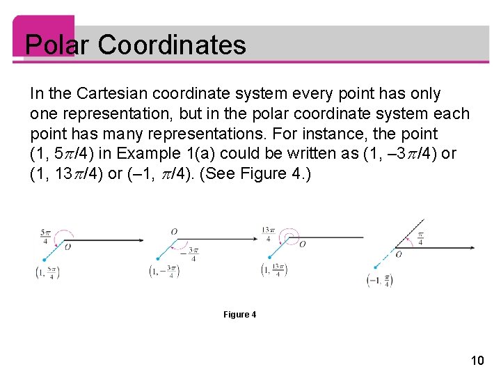
Polar Coordinates In the Cartesian coordinate system every point has only one representation, but in the polar coordinate system each point has many representations. For instance, the point (1, 5 /4) in Example 1(a) could be written as (1, – 3 /4) or (1, 13 /4) or (– 1, /4). (See Figure 4. ) Figure 4 10

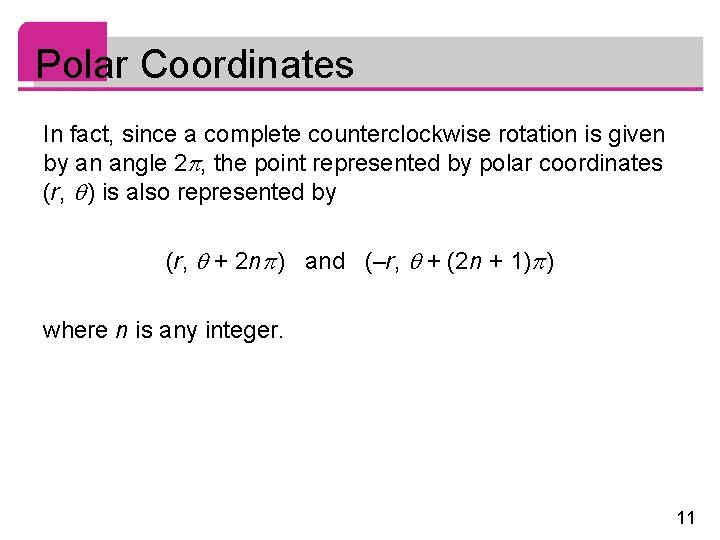
Polar Coordinates In fact, since a complete counterclockwise rotation is given by an angle 2 , the point represented by polar coordinates (r, ) is also represented by (r, + 2 n ) and (–r, + (2 n + 1) ) where n is any integer. 11

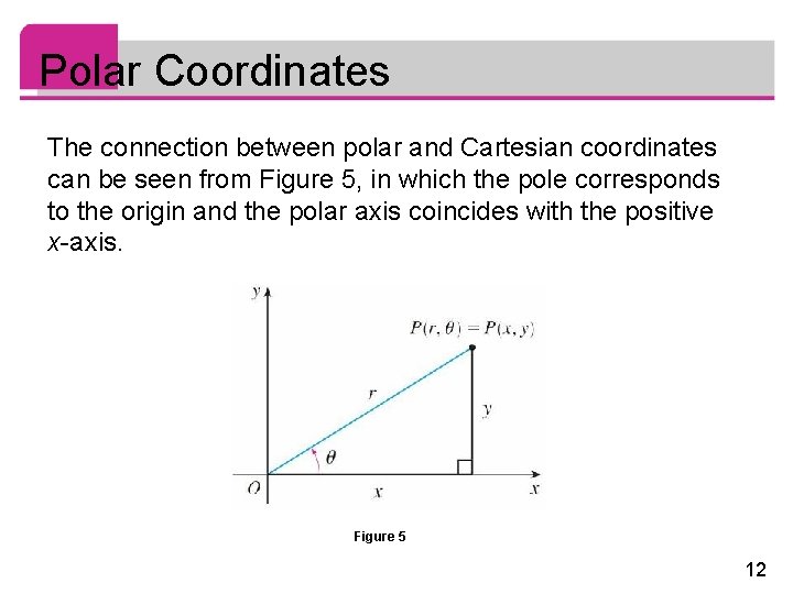
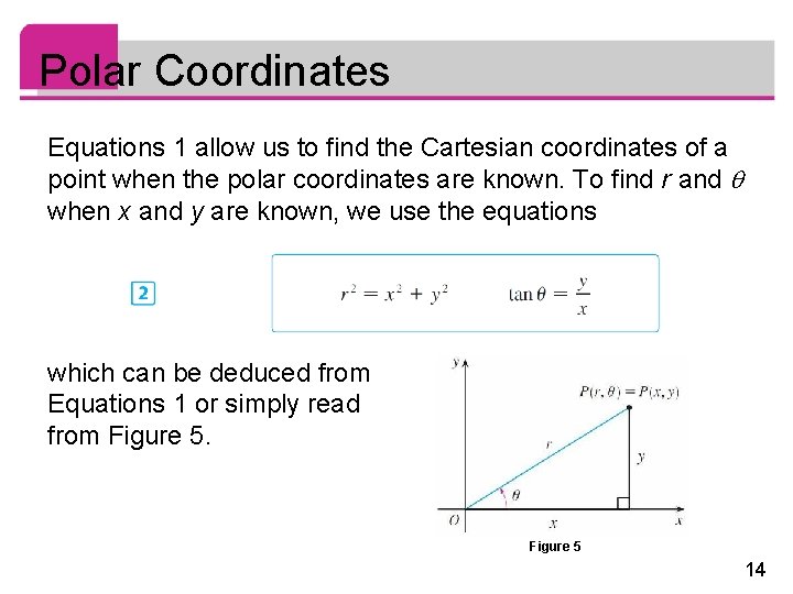
Polar Coordinates The connection between polar and Cartesian coordinates can be seen from Figure 5, in which the pole corresponds to the origin and the polar axis coincides with the positive x-axis. Figure 5 12

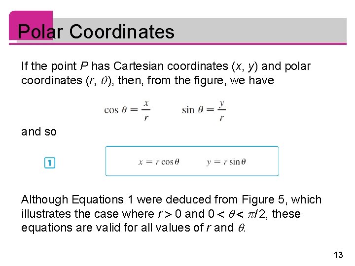
Polar Coordinates If the point P has Cartesian coordinates (x, y) and polar coordinates (r, ), then, from the figure, we have and so Although Equations 1 were deduced from Figure 5, which illustrates the case where r 0 and 0 / 2, these equations are valid for all values of r and . 13

Polar Coordinates Equations 1 allow us to find the Cartesian coordinates of a point when the polar coordinates are known. To find r and when x and y are known, we use the equations which can be deduced from Equations 1 or simply read from Figure 5 14

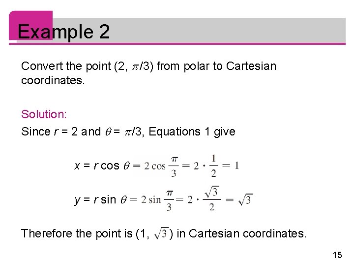
Example 2 Convert the point (2, /3) from polar to Cartesian coordinates. Solution: Since r = 2 and = /3, Equations 1 give x = r cos y = r sin Therefore the point is (1, ) in Cartesian coordinates. 15

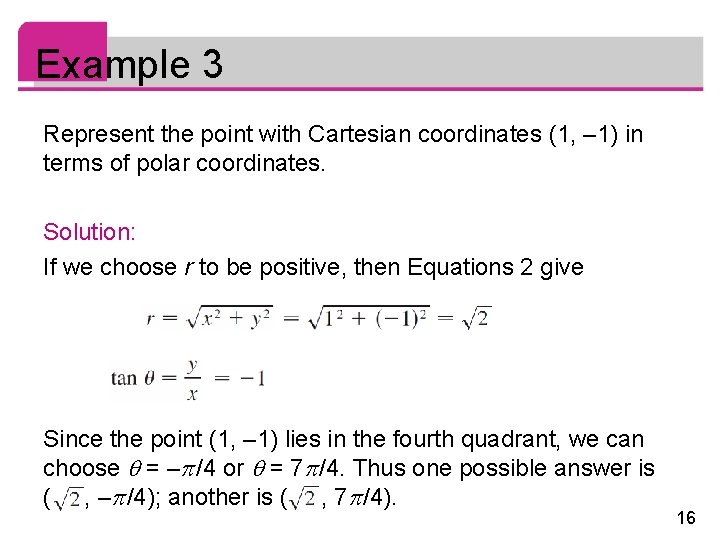
Example 3 Represent the point with Cartesian coordinates (1, – 1) in terms of polar coordinates. Solution: If we choose r to be positive, then Equations 2 give Since the point (1, – 1) lies in the fourth quadrant, we can choose = – /4 or = 7 /4. Thus one possible answer is ( , – /4); another is ( , 7 /4). 16

Polar Coordinates Note Equations 2 do not uniquely determine when x and y are given because, as increases through the interval 0 2 , each value of tan occurs twice. Therefore, in converting from Cartesian to polar coordinates, it’s not good enough just to find r and that satisfy Equations 2. As in Example 3, we must choose so that the point (r, ) lies in the correct quadrant. 17

Polar Curves 18

Polar Curves The graph of a polar equation r = f ( ), or more generally F (r, ) = 0, consists of all points P that have at least one polar representation (r, ) whose coordinates satisfy the equation. 19

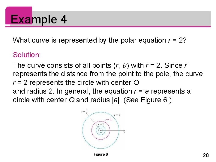
Example 4 What curve is represented by the polar equation r = 2? Solution: The curve consists of all points (r, ) with r = 2. Since r represents the distance from the point to the pole, the curve r = 2 represents the circle with center O and radius 2. In general, the equation r = a represents a circle with center O and radius |a|. (See Figure 6. ) Figure 6 20

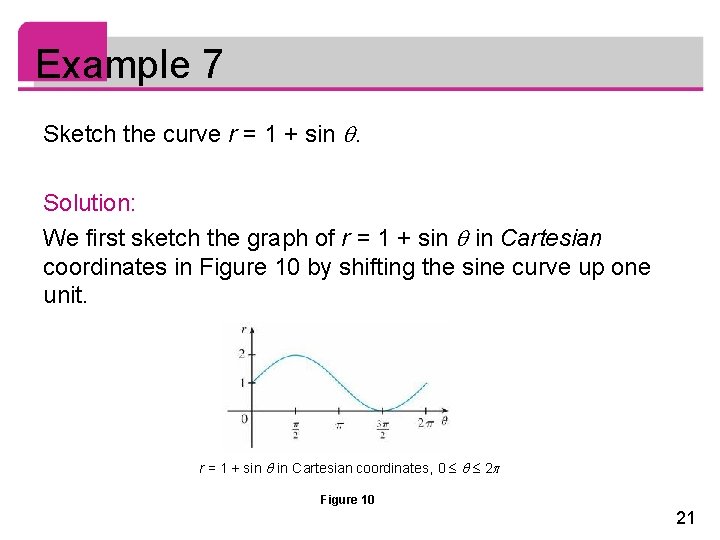
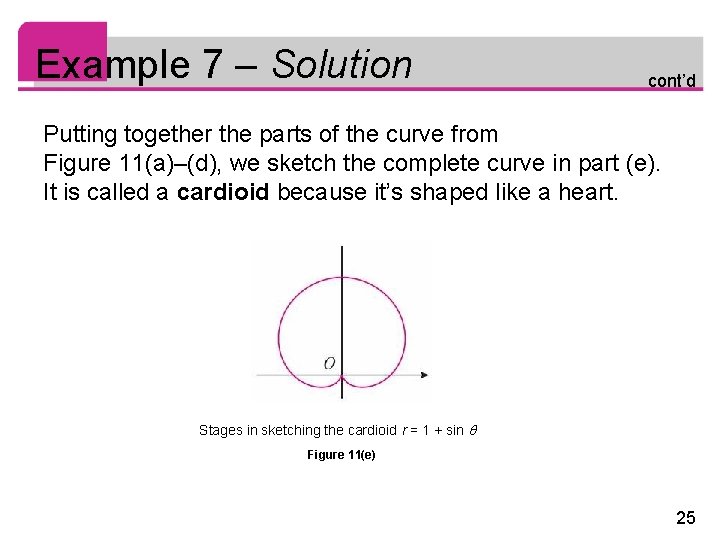
Example 7 Sketch the curve r = 1 + sin . Solution: We first sketch the graph of r = 1 + sin in Cartesian coordinates in Figure 10 by shifting the sine curve up one unit. r = 1 + sin in Cartesian coordinates, 0 2 Figure 10 21

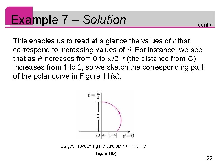
Example 7 – Solution cont’d This enables us to read at a glance the values of r that correspond to increasing values of . For instance, we see that as increases from 0 to /2, r (the distance from O) increases from 1 to 2, so we sketch the corresponding part of the polar curve in Figure 11(a). Stages in sketching the cardioid r = 1 + sin Figure 11(a) 22

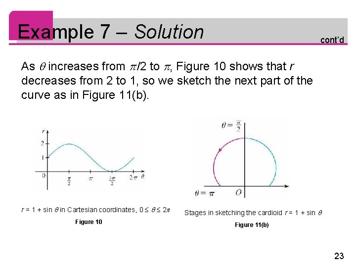
Example 7 – Solution cont’d As increases from /2 to , Figure 10 shows that r decreases from 2 to 1, so we sketch the next part of the curve as in Figure 11(b). r = 1 + sin in Cartesian coordinates, 0 2 Figure 10 Stages in sketching the cardioid r = 1 + sin Figure 11(b) 23

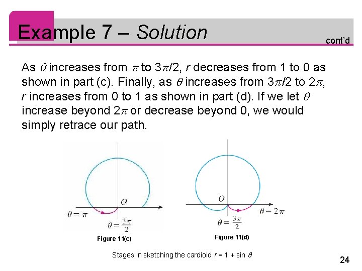
Example 7 – Solution cont’d As increases from to 3 /2, r decreases from 1 to 0 as shown in part (c). Finally, as increases from 3 /2 to 2 , r increases from 0 to 1 as shown in part (d). If we let increase beyond 2 or decrease beyond 0, we would simply retrace our path. Figure 11(c) Figure 11(d) Stages in sketching the cardioid r = 1 + sin 24

Example 7 – Solution cont’d Putting together the parts of the curve from Figure 11(a)–(d), we sketch the complete curve in part (e). It is called a cardioid because it’s shaped like a heart. Stages in sketching the cardioid r = 1 + sin Figure 11(e) 25

Polar Curves The remainder of the curve is drawn in a similar fashion, with the arrows and numbers indicating the order in which the portions are traced out. The resulting curve has four loops and is called a four-leaved rose. 26

Symmetry 27

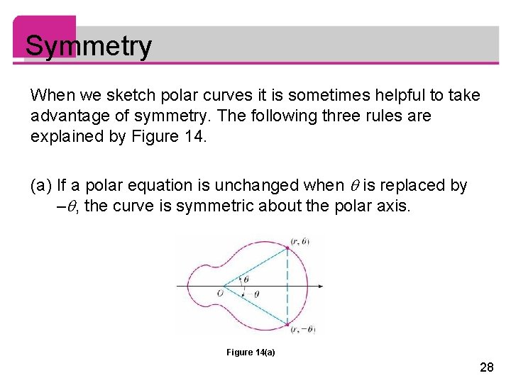
Symmetry When we sketch polar curves it is sometimes helpful to take advantage of symmetry. The following three rules are explained by Figure 14. (a) If a polar equation is unchanged when is replaced by – , the curve is symmetric about the polar axis. Figure 14(a) 28

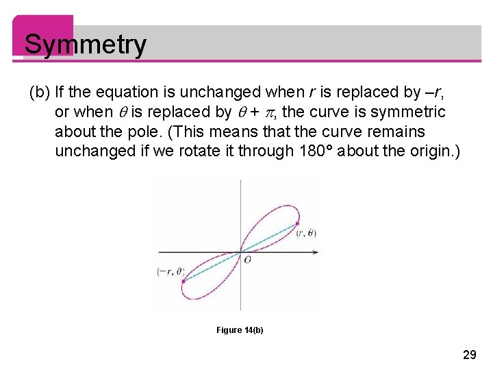
Symmetry (b) If the equation is unchanged when r is replaced by –r, or when is replaced by + , the curve is symmetric about the pole. (This means that the curve remains unchanged if we rotate it through 180° about the origin. ) Figure 14(b) 29

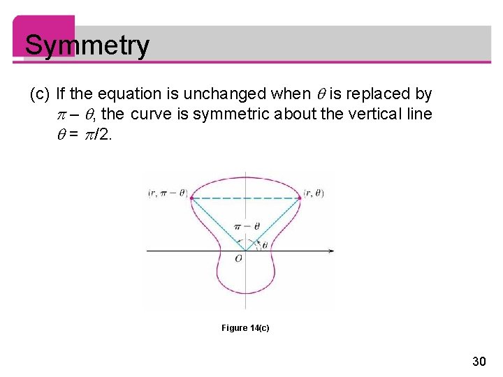
Symmetry (c) If the equation is unchanged when is replaced by – , the curve is symmetric about the vertical line = /2. Figure 14(c) 30

Symmetry The curves in Example 7 is symmetric about = /2 because sin( – ) = sin and cos 2( – ) = cos 2. The four-leaved rose is also symmetric about the pole. These symmetry properties could have been used in sketching the curves. 31

Tangents to Polar Curves 32

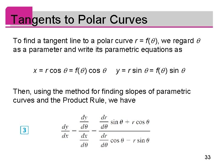
Tangents to Polar Curves To find a tangent line to a polar curve r = f ( ), we regard as a parameter and write its parametric equations as x = r cos = f ( ) cos y = r sin = f ( ) sin Then, using the method for finding slopes of parametric curves and the Product Rule, we have 33

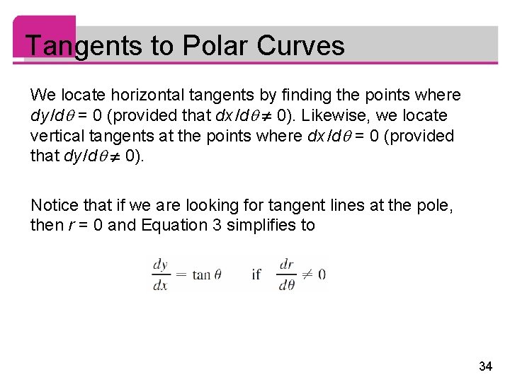
Tangents to Polar Curves We locate horizontal tangents by finding the points where dy /d = 0 (provided that dx /d 0). Likewise, we locate vertical tangents at the points where dx /d = 0 (provided that dy /d 0). Notice that if we are looking for tangent lines at the pole, then r = 0 and Equation 3 simplifies to 34

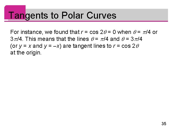
Tangents to Polar Curves For instance, we found that r = cos 2 = 0 when = /4 or 3 /4. This means that the lines = /4 and = 3 /4 (or y = x and y = –x) are tangent lines to r = cos 2 at the origin. 35

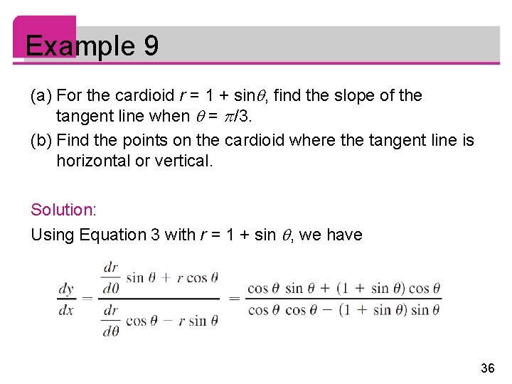
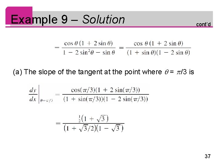
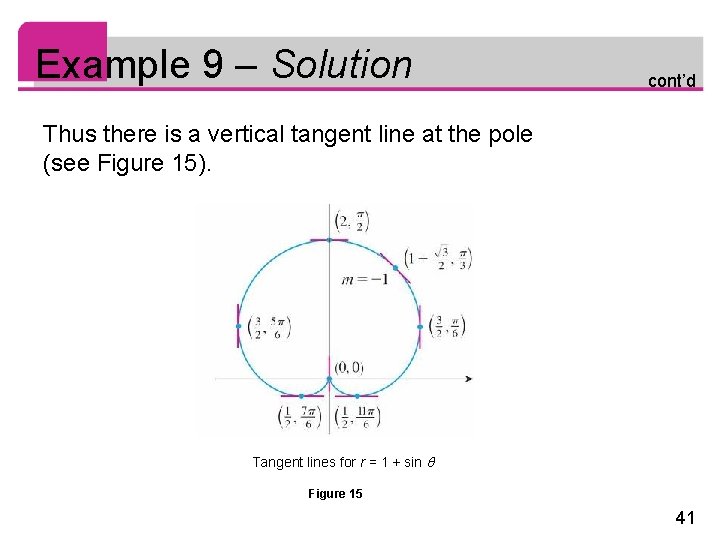
Example 9 (a) For the cardioid r = 1 + sin , find the slope of the tangent line when = /3. (b) Find the points on the cardioid where the tangent line is horizontal or vertical. Solution: Using Equation 3 with r = 1 + sin , we have 36

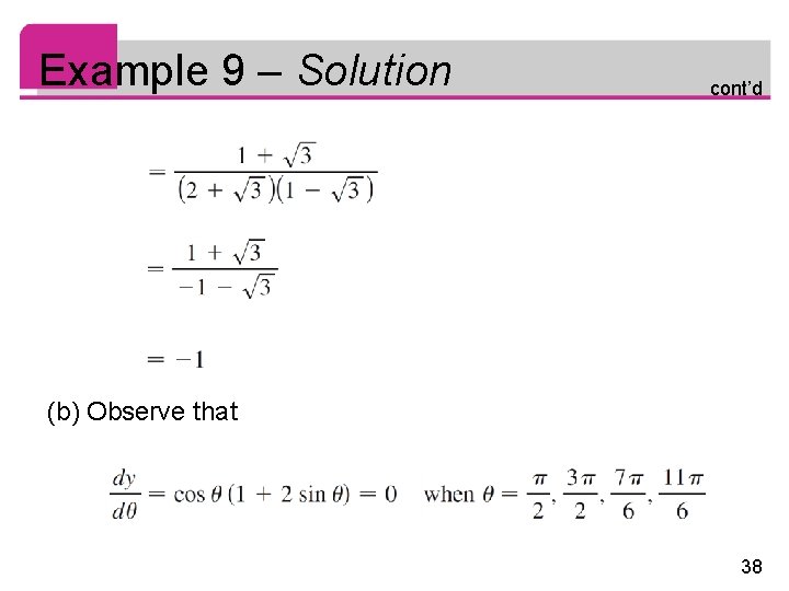
Example 9 – Solution cont’d (a) The slope of the tangent at the point where = /3 is 37

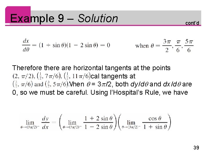
Example 9 – Solution cont’d (b) Observe that 38

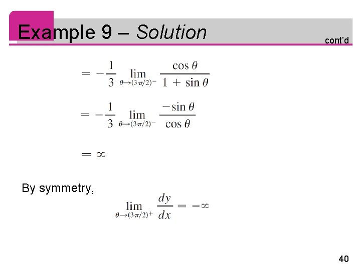
Example 9 – Solution cont’d Therefore there are horizontal tangents at the points and vertical tangents at When = 3 /2, both dy /d and dx /d are 0, so we must be careful. Using l’Hospital’s Rule, we have 39

Example 9 – Solution cont’d By symmetry, 40

Example 9 – Solution cont’d Thus there is a vertical tangent line at the pole (see Figure 15). Tangent lines for r = 1 + sin Figure 15 41

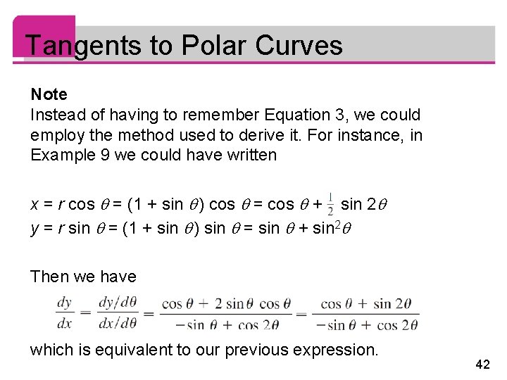
Tangents to Polar Curves Note Instead of having to remember Equation 3, we could employ the method used to derive it. For instance, in Example 9 we could have written x = r cos = (1 + sin ) cos = cos + sin 2 y = r sin = (1 + sin ) sin = sin + sin 2 Then we have which is equivalent to our previous expression. 42

Graphing Polar Curves with Graphing Devices 43

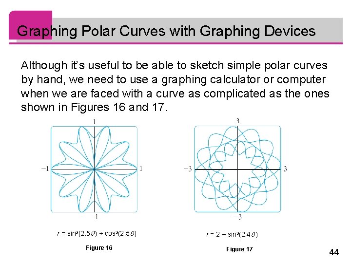
Graphing Polar Curves with Graphing Devices Although it’s useful to be able to sketch simple polar curves by hand, we need to use a graphing calculator or computer when we are faced with a curve as complicated as the ones shown in Figures 16 and 17. r = sin 3(2. 5 ) + cos 3(2. 5 ) Figure 16 r = 2 + sin 3(2. 4 ) Figure 17 44

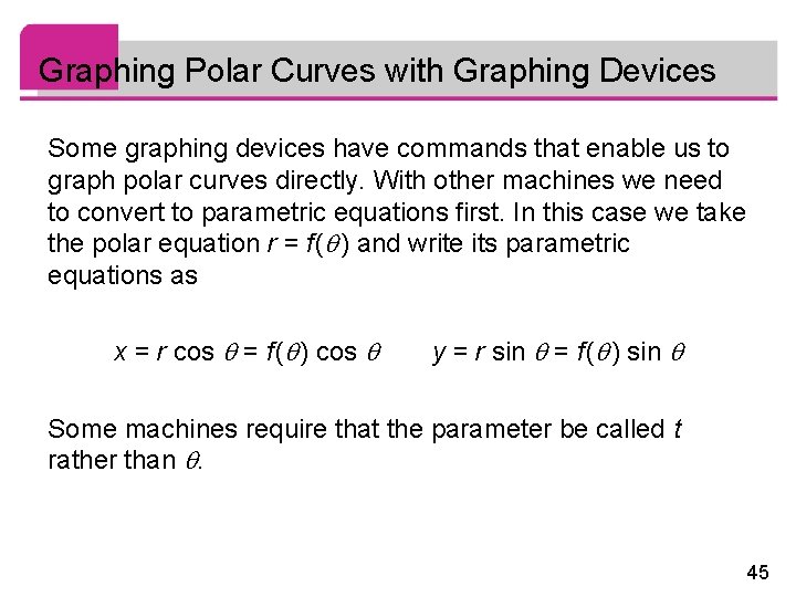
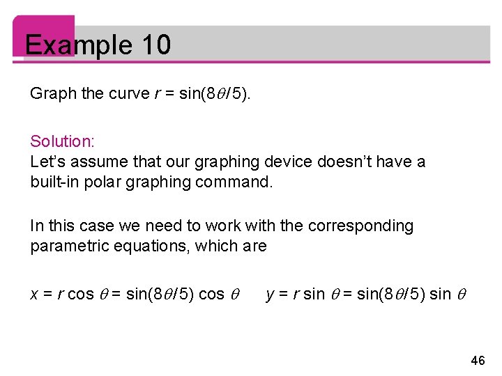
Graphing Polar Curves with Graphing Devices Some graphing devices have commands that enable us to graph polar curves directly. With other machines we need to convert to parametric equations first. In this case we take the polar equation r = f ( ) and write its parametric equations as x = r cos = f ( ) cos y = r sin = f ( ) sin Some machines require that the parameter be called t rather than . 45

Example 10 Graph the curve r = sin(8 / 5). Solution: Let’s assume that our graphing device doesn’t have a built-in polar graphing command. In this case we need to work with the corresponding parametric equations, which are x = r cos = sin(8 / 5) cos y = r sin = sin(8 / 5) sin 46

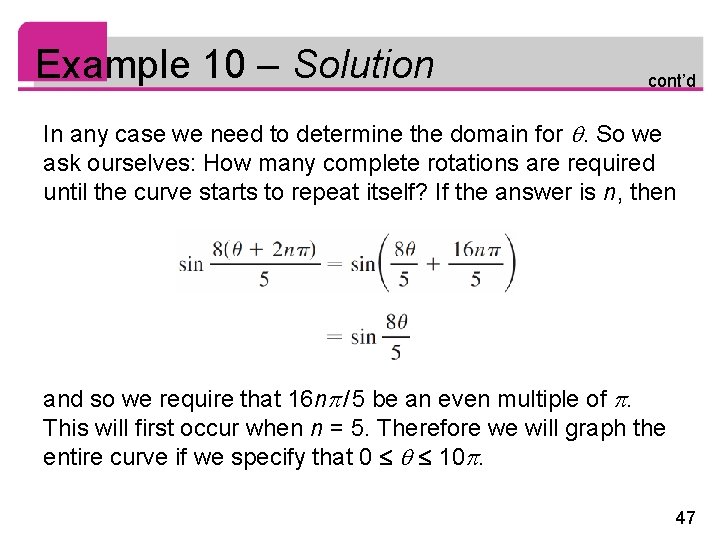
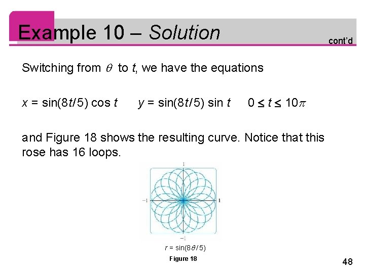
Example 10 – Solution cont’d In any case we need to determine the domain for . So we ask ourselves: How many complete rotations are required until the curve starts to repeat itself? If the answer is n, then and so we require that 16 n / 5 be an even multiple of . This will first occur when n = 5. Therefore we will graph the entire curve if we specify that 0 10. 47

Example 10 – Solution cont’d Switching from to t, we have the equations x = sin(8 t / 5) cos t y = sin(8 t / 5) sin t 0 t 10 and Figure 18 shows the resulting curve. Notice that this rose has 16 loops. r = sin(8 / 5) Figure 18 48