Association Rule Mining on Remotely Sensed Imagery Using

Association Rule Mining on Remotely Sensed Imagery Using Peano-trees (P-trees) Qin Ding, Qiang Ding, and William Perrizo Computer Science Department North Dakota State University, USA May 2002 (P-tree technology is patent pending by NDSU)

Outline l Concepts – Association Rule Mining – Market Basket Data – Remotely Sensed Imagery (RSI) data – Peano Count Trees (P-trees) Association rule mining on RSI data using P-trees l Performance analysis l Conclusion l

Association Rule Mining l Originally proposed for market basket data. Given – A set of items I = {i 1, i 2, …im} (e. g. , items purchasable in a market) – A set of transactions D (e. g. , customers checking out = id + itemset) l An association rule is X=>Y, where X, Y are disjoint itemsets – X, Y are consider as events. l E. g. , X is the event that a transaction contains X. l X=>Y is the event: “if t contains X, then it contains Y” l X is called the antecedent, Y is called the consequent. l Two measures: support (% trans containing X Y) and confidence (% of those transactions containing X which also contain Y) l Given minimum thresholds, minsup and minconf, – Find the frequent itemsets which have support above minsup. – Derive all rules supported by frequent sets, with confidence above minconf.

Association rule mining on RSI data l RSI data can be viewed as a relational table – Each band (column) is an attribute (for simplicity we assume all values are bytes) – Each pixel (row) is a transaction. – Each interval in each band is an item. – Row/column or longitude/latitude is the primary key l ARM task on RSI data – To mine implicit relations among different bands, for example, relations among spectral bands and yield. l Example Rule (NDVI): NIR[192, 255] ^ RED[0, 63] => Yield[128, 255]

Important ARM Algorithms l Apriori – stepwise algorithm l DHP (Direct Hashing and Pruning) – hash itemset counts and prune transactions l Partition – divide the database into small partitions such that each can be processed independently and efficiently in memory. l DIC (Dynamic Itemset Counting) – overlap the counting of candidate itemsets at different points during a scan. FP-growth – uses Frequent Pattern tree (FP-tree) to optimize candidate generation. l Others… l

Remotely Sensed Imagery (RSI) Data l Satellite image – TM (Thematic Mapper) imagery (6, 7 or 8 bands) l l TM is Landsat satellite imagery covering the earth every 18 days since 1972. ETM+ (Landsat-7) contains 8 bands – 7 VIR bands (Blue, Green, Red, NIR, MIR, TIR, MIR 2) – 1 Panchromatic band (PC). l Aerial photography – TIFF (3 bands: Blue, Green, Red) l Ground data – Yield, Moisture, Nitrate, Temperature, Elevation, etc

Precision Agriculture Dataset: TIFF Image and related Bands (1320× 1320) RGB Yield Moisture Nitrate

As a relation x y RG BYM N 812 812 812 812 812 812 812 812 445 446 447 448 449 450 451 452 453 454 455 456 457 458 459 460 461 462 463 464 465 466 467 468 469 470 471 472 473 474 43 43 47 50 51 46 33 30 41 40 43 42 40 40 38 34 39 36 42 40 39 40 30 33 35 30 30 60 58 60 63 69 73 68 65 63 53 49 55 55 56 52 58 66 59 51 53 54 57 59 68 56 45 57 58 54 57 59 50 52 54 58 54 54 50 47 54 57 52 52 45 47 47 55 63 57 48 43 50 57 43 45 62 63 52 146 146 146 146 146 145 145 145 145 83 83 83 83 83 82 82 82 188 187 186 185 184 183 182 181 180 179 178 177 176 175 174 173 172 172 172 173 173 x: Row y: Column R: Red G: Green B: Blue Y: Yield M: Moisture N: Nitrate

Spatial Data Formats 254 (1111 1110) BAND-1 127 (0111 1111) 37 (0010 0101) BAND-2 240 (1111 0000) 14 (0000 1110) 193 (1100 0001) 200 (1100 1000) 19 (0001 0011) BSQ format (2 files) Band 1: 254 127 14 193 Band 2: 37 240 200 19

Spatial Data Formats 254 (1111 1110) BAND-1 127 (0111 1111) 37 (0010 0101) BAND-2 240 (1111 0000) 14 (0000 1110) 193 (1100 0001) 200 (1100 1000) 19 (0001 0011) BSQ format (2 files) BIL format (1 file) Band 1: 254 127 14 193 Band 2: 37 240 200 19 254 127 37 240 14 193 200 19

Spatial Data Formats 254 (1111 1110) BAND-1 127 (0111 1111) 37 (0010 0101) BAND-2 240 (1111 0000) 14 (0000 1110) 193 (1100 0001) 200 (1100 1000) 19 (0001 0011) BSQ format (2 files) BIL format (1 file) BIP format (1 file) Band 1: 254 127 14 193 Band 2: 37 240 200 19 254 127 37 240 14 193 200 19 254 37 127 240 14 200 193 19

Spatial Data Formats 254 (1111 1110) BAND-1 127 (0111 1111) 37 (0010 0101) BAND-2 240 (1111 0000) 14 (0000 1110) 193 (1100 0001) 200 (1100 1000) 19 (0001 0011) BSQ format (2 files) BIL format (1 file) BIP format (1 file) Band 1: 254 127 14 193 Band 2: 37 240 200 19 254 127 37 240 14 193 200 19 254 37 127 240 14 200 193 19 b. SQ format (16 files) B 11 B 12 B 13 B 14 B 15 1 1 1 0 0 1 1 1 0 0 0 B 16 B 17 B 18 B 21 B 22 B 23 1 1 0 0 0 1 1 1 1 1 0 0 0 B 24 B 25 B 26 0 0 1 1 0 0 0 1 0 0 B 27 B 28 0 1 0 0 1 1

Peano Count Tree (P-tree) l P-tree represents RSI data bit-by-bit in a recursive quadrant-by-quadrant arrangement. l P-trees are a lossless compressed representation of the original data.

An example 2 -D a P-tree b. SQ file 1 1 1 1 1 0 0 0 1 1 1 1 1 1 1 1 1 1 b. SQ file arranged as a spatial dataset (2 -D raster order) 11 11 01 11 11 10 11 11 00 00 10 00 00 39 16 8 3 0 0 15 4 1 4 4 3 4 1 1 1 0 0 0 1 1 0 1 Quadrant-based, Pure (Pure-1/Pure-0) quadrant l Peano or Z-ordering l Root Count l

Peano Mask Tree (PM-tree) 11 11 01 l 11 11 11 10 11 11 00 00 10 00 00 m m 1 m 0 m 1 1 0 0 0 1 1 0 1 Truth-Trees (1 if condition is true of quadrant, else 0 – E. g. , Pure-1 and Pure-0 Trees – All are lossless compressed representations of the dataset 0

001 11 11 11 11 10 11 11 11 00 00 00 10 11 11 55 0 16 2 8 3 Peano or Z-ordering l Pure-1/Pure-0 quadrant l Root Count ( 111, 001 ) 0 4 1 4 3 15 2 4 3 16 4 3 1 1 1 0 0 0 1 1 0 1 l ( 7, 1 ) 1 2. 2. 3 Ø Level Ø Fan-out Ø QID (Quadrant ID) 10. 11

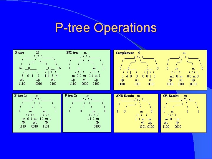
Ptree ANDing Operation PM-tree 1: m ______/ / ______ / / 1 m m 1 / / m 0 1 m 1 //| 1110 0010 1101 PM-tree 2: m ______/ / ______ / / 1 0 m 0 / / 11 1 m //| 0100 Result: m ____ / / ___ / ____ / / / 1 0 m 0 / | 1 1 m m //| 1101 0100 Depth-first Pure-1 path code 0 101 102 12 132 20 21 220 221 223 23 3 & 0 20 21 22 231 0 0 20 20 21 21 220 221 223 22 23 231 RESULT 0 20 21 220 221 223 231

Various P-trees AND, OR, COMPLEMENT Basic P-trees Pi, j AND, OR COMPLEMENT Value P-trees Pi(v) OR AND Tuple P-trees P(v 1, v 2, …, vn) Predicate P-trees P(p) Interval P-trees Pi(v 1, v 2) AND OR Cube P-trees P([v 11, v 12], …, [v. N 1, v. N 2])

Association Rule Mining on RSI Data using P-trees l Admissible Itemsets (Asets ) – Asets are itemsets of the form, Int 1 Int 2 . . . Intn = Π i=1. . . n Inti , where Inti is an interval of values in Bandi (some of which may be the full value range). – Example: Aset {[01, 01]1, [11, 11]2} l P-ARM algorithm l Pruning techniques

P-ARM algorithm Procedure P-ARM { Data_Discretization; F 1 = {frequent 1 -Asets}; For (k=2; F k-1 ) do begin Ck = p-gen(F k-1); Forall candidate Asets c Ck do c. count = AND_rootcount(c); Fk = {c Ck | c. count >= minsup} end Answer = k Fk } • F 1 is determined directly from P-tree root counnts and pruning techniques rather than transaction database scan. • The p-gen function differs from the apriori-gen function in Apriori by using some pruning techniques. • • The AND_rootcount function is used to calculate Aset counts directly by ANDing the appropriate basic Ptrees instead of scanning the transaction databases. The support count for Aset {B 1[0, 64), B 2[64, 127)} (or {[00, 00]1, [01, 01]2}) is the root count of P 1(00) AND P 2(01).

Pruning Techniques l Band-based pruning – An itemset with two items from the same band will have support zero. l Constraint-base pruning – E. g. , specify yield as the only consequent band of interest. – Note: in the performance comparisons we did not use this pruning technique (to maintain fairness, since it is hard to implement in other alogrithms) l Bit-based pruning for multi-level rules – if Aset [128, 255] (or [1, 1]2) is not frequent, then the Aset [128, 191] (or [10, 10]2) and [192, 255] (or [11, 11]2) cannot be frequent either. l Others

P-ARM versus Apriori 1, 742, 400 pixels (transactions) Scalability with support threshold

P-ARM versus Apriori (cont. ) Support threshold =10% Scalability with number of transactions

P-ARM versus FP-growth Run time (Sec. ) 800 17, 424, 000 pixels (transactions) 1, 742, 400 pixels (transactions) 700 600 P-ARM 500 400 FP-growth 300 200 100 0 10% 30% 50% 70% 90% Support threshold Scalability with support threshold

P-ARM versus FP-growth (cont. ) Support threshold =10% Scalability with the number of transactions

Conclusion l A model for association rule mining on RSI data – P-trees facilitate fast calculation of support – P-trees facilitates significant pruning techniques l Applications other than precision agriculture – Flood prediction and monitoring – Community and regional planning – Virtual archeology – Mineral exploration – Bioinformatics/Genomics – VLSI design