Sorting Quick Sort Shell Sort Counting Sort Radix

Sorting Quick Sort, Shell Sort, Counting Sort, Radix Sort AND Bucket Sort

Motivation of Sorting �Sorting algorithms contain interesting and important ideas for code optimization as well as algorithm design.

Merge Sort Last time we talked about Merge Sort ◦ Recursively calls: Merge. Sort(1 st half of list) Merge. Sort(2 nd half of list) Then Merges results

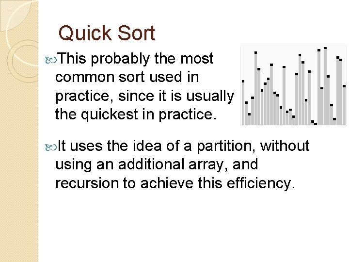
Quick Sort This probably the most common sort used in practice, since it is usually the quickest in practice. It uses the idea of a partition, without using an additional array, and recursion to achieve this efficiency.

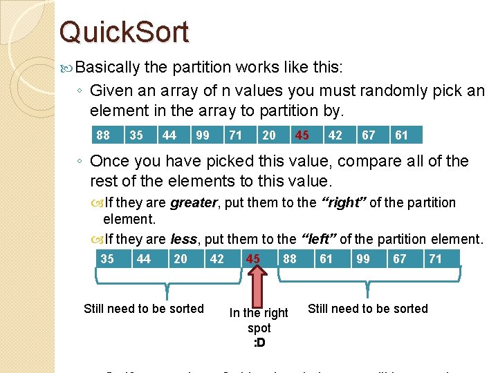
Quick. Sort Basically the partition works like this: ◦ Given an array of n values you must randomly pick an element in the array to partition by. 88 35 44 99 71 20 45 42 67 61 ◦ Once you have picked this value, compare all of the rest of the elements to this value. If they are greater, put them to the “right” of the partition element. If they are less, put them to the “left” of the partition element. 35 44 20 Still need to be sorted 42 45 88 In the right spot : D 61 99 67 Still need to be sorted 71

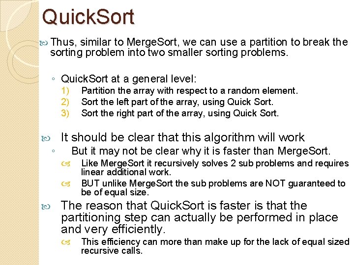
Quick. Sort Thus, similar to Merge. Sort, we can use a partition to break the sorting problem into two smaller sorting problems. ◦ Quick. Sort at a general level: 1) 2) 3) ◦ It should be clear that this algorithm will work But it may not be clear why it is faster than Merge. Sort. Partition the array with respect to a random element. Sort the left part of the array, using Quick Sort the right part of the array, using Quick Sort. Like Merge. Sort it recursively solves 2 sub problems and requires linear additional work. BUT unlike Merge. Sort the sub problems are NOT guaranteed to be of equal size. The reason that Quick. Sort is faster is that the partitioning step can actually be performed in place and very efficiently. This efficiency can more than make up for the lack of equal sized recursive calls.

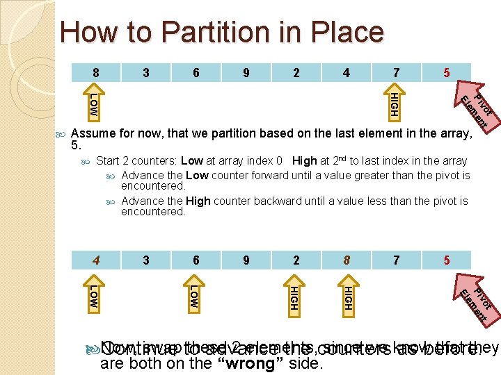
How to Partition in Place 8 3 6 9 2 4 5 t vo t Pi men e El HIGH LOW 7 Assume for now, that we partition based on the last element in the array, 5. Start 2 counters: Low at array index 0 High at 2 nd to last index in the array Advance the Low counter forward until a value greater than the pivot is encountered. Advance the High counter backward until a value less than the pivot is encountered. 6 9 4 8 7 5 t vo t Pi men e El LOW 2 HIGH 3 HIGH 8 4 swap to these 2 elements, since we know that they Now, Continue advance the counters as before. are both on the “wrong” side.

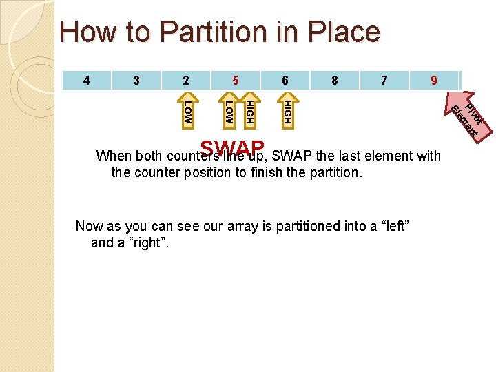
How to Partition in Place 44 33 226 59 662 88 77 95 Now as you can see our array is partitioned into a “left” and a “right”. t vo t Pi men e El HIGH LOW SWAP When both counters line up, SWAP the last element with the counter position to finish the partition.

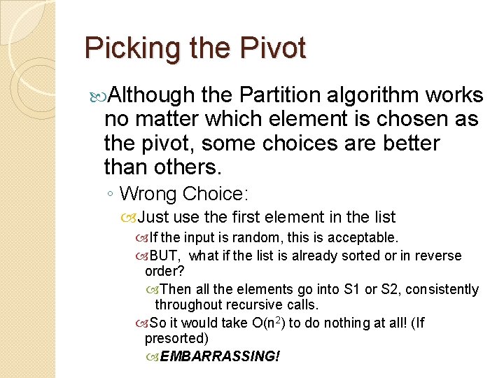
Picking the Pivot Although the Partition algorithm works no matter which element is chosen as the pivot, some choices are better than others. ◦ Wrong Choice: Just use the first element in the list If the input is random, this is acceptable. BUT, what if the list is already sorted or in reverse order? Then all the elements go into S 1 or S 2, consistently throughout recursive calls. So it would take O(n 2) to do nothing at all! (If presorted) EMBARRASSING!

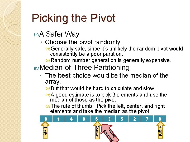
Picking the Pivot A Safer Way ◦ Choose the pivot randomly Generally safe, since it’s unlikely the random pivot would consistently be a poor partition. Random number generation is generally expensive. Median-of-Three Partitioning ◦ The best choice would be the median of the array. But that would be hard to calculate and slow. A good estimate is to pick 3 elements and use the median of those as the pivot. The rule of thumb: Pick the left, center, and right elements and take the median as the pivot. 8 1 4 9 6 3 5 2 7 0 Right t vo t Pi men e El Center Left

Analysis of Quicksort Shown on the board

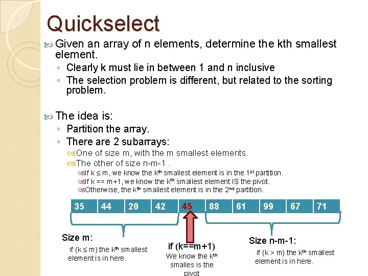
Quickselect Given an array of n elements, determine the kth smallest element. ◦ Clearly k must lie in between 1 and n inclusive ◦ The selection problem is different, but related to the sorting problem. The idea is: ◦ Partition the array. ◦ There are 2 subarrays: One of size m, with the m smallest elements. The other of size n-m-1. If k ≤ m, we know the kth smallest element is in the 1 st partition. If k == m+1, we know the kth smallest element IS the pivot. Otherwise, the kth smallest element is in the 2 nd partition. 35 44 20 Size m: kth if (k ≤ m) the smallest element is in here. 42 45 88 if (k==m+1) We know the kth smalles is the pivot 61 99 67 71 Size n-m-1: if (k > m) the kth smallest element is in here.

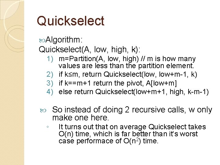
Quickselect Algorithm: Quickselect(A, low, high, k): 1) m=Partition(A, low, high) // m is how many values are less than the partition element. 2) if k≤m, return Quickselect(low, low+m-1, k) 3) if k==m+1 return the pivot, A[low+m] 4) else return Quickselect(low+m+1, high, k-m-1) ◦ So instead of doing 2 recursive calls, w only make one here. It turns out that on average Quickselect takes O(n) time, which is far better than it’s worst case performace of O(n 2) time.

Quickselect Analysis Shown on the board

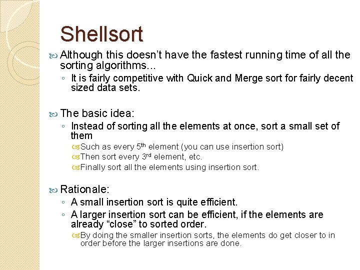
Shellsort Although this doesn’t have the fastest running time of all the sorting algorithms. . . ◦ It is fairly competitive with Quick and Merge sort for fairly decent sized data sets. The basic idea: ◦ Instead of sorting all the elements at once, sort a small set of them Such as every 5 th element (you can use insertion sort) Then sort every 3 rd element, etc. Finally sort all the elements using insertion sort. Rationale: ◦ A small insertion sort is quite efficient. ◦ A larger insertion sort can be efficient, if the elements are already “close” to sorted order. By doing the smaller insertion sorts, the elements do get closer to in order before the larger insertions are done.

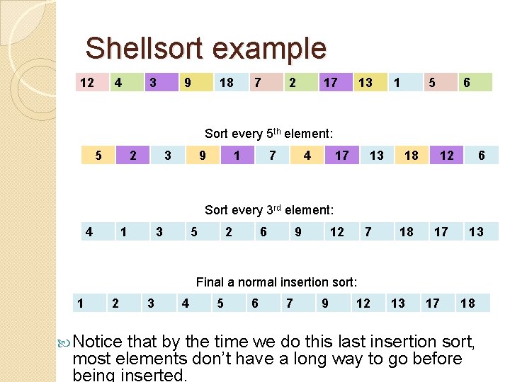
Shellsort example 12 12 44 33 99 18 18 77 22 17 17 13 13 11 55 66 Sort every 5 th element: 5 2 3 9 1 7 4 17 13 18 12 6 Sort every 3 rd element: 4 1 3 5 2 6 9 12 7 18 17 13 Final a normal insertion sort: 1 2 Notice 3 4 5 6 7 9 12 13 17 18 that by the time we do this last insertion sort, most elements don’t have a long way to go before being inserted.

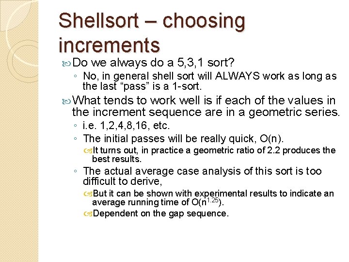
Shellsort – choosing increments Do we always do a 5, 3, 1 sort? ◦ No, in general shell sort will ALWAYS work as long as the last “pass” is a 1 -sort. What tends to work well is if each of the values in the increment sequence are in a geometric series. ◦ i. e. 1, 2, 4, 8, 16, etc. ◦ The initial passes will be really quick, O(n). It turns out, in practice a geometric ratio of 2. 2 produces the best results. ◦ The actual average case analysis of this sort is too difficult to derive, But it can be shown with experimental results to indicate an average running time of O(n 1. 25). Dependent on the gap sequence.

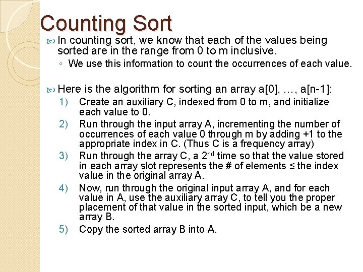
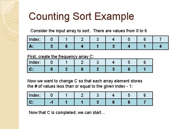
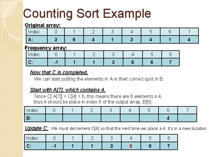
Counting Sort In counting sort, we know that each of the values being sorted are in the range from 0 to m inclusive. ◦ We use this information to count the occurrences of each value. Here 1) 2) 3) 4) 5) is the algorithm for sorting an array a[0], …, a[n-1]: Create an auxiliary C, indexed from 0 to m, and initialize each value to 0. Run through the input array A, incrementing the number of occurrences of each value 0 through m by adding +1 to the appropriate index in C. (Thus C is a frequency array) Run through the array C, a 2 nd time so that the value stored in each array slot represents the # of elements ≤ the index value in the original array A. Now, run through the original input array A, and for each value in A, use the auxiliary array C, to tell you the proper placement of that value in the sorted input, which be a new array B. Copy the sorted array B into A.

Counting Sort Example Consider the input array to sort. There are values from 0 to 6 Index: 0 1 2 3 4 5 6 7 A: 3 6 4 1 3 4 1 4 First, create the frequency array C: Index: 0 1 2 3 4 5 6 3 0 1 C: 0 2 Now we want to change C so that each array element stores the # of values less than or equal to the given index - 1: Index: 0 1 2 3 4 5 6 C: -1 1 1 3 6 6 7 Now that C is completed, we can start…

Counting Sort Example Original array: Index: 0 1 2 3 4 5 6 7 A: 3 6 4 1 3 4 1 4 Frequency array: Index: 0 1 2 3 4 5 6 C: -1 1 1 3 6 6 7 Now that C is completed, We can start putting the elements in A in their correct spot in B: Start with A[7], which contains 4. Since C[ A[7]] = C[4] = 6, this means there are 6 elements ≤ 4, thus 4 should be place in index 6 of the output array, B[6]: Index: 0 1 2 3 4 5 B: 6 7 4 Update C: We must decrement C[4] so that the next time we place a 4, it’s in a new location. Index: 0 1 2 3 4 5 6 C: -1 1 1 3 5 6 7

Counting Sort Example Finish on the board

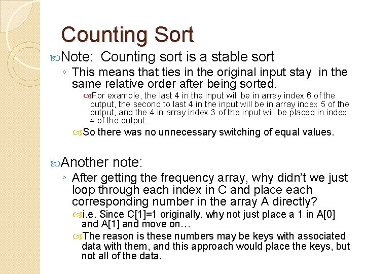
Counting Sort Note: Counting sort is a stable sort ◦ This means that ties in the original input stay in the same relative order after being sorted. For example, the last 4 in the input will be in array index 6 of the output, the second to last 4 in the input will be in array index 5 of the output, and the 4 in array index 3 of the input will be placed in index 4 of the output. So there was no unnecessary switching of equal values. Another note: ◦ After getting the frequency array, why didn’t we just loop through each index in C and place each corresponding number in the array A directly? i. e. Since C[1]=1 originally, why not just place a 1 in A[0] and A[1] and move on… The reason is these numbers may be keys with associated data with them, and this approach would place the keys, but not all of the data.

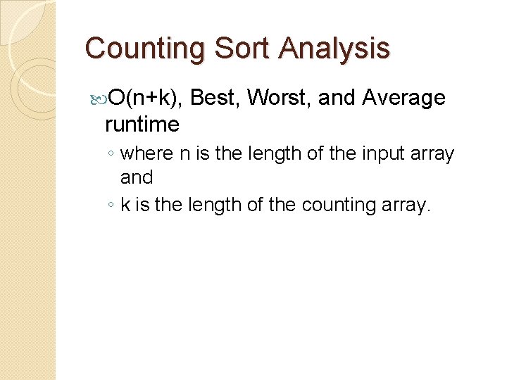
Counting Sort Analysis O(n+k), Best, Worst, and Average runtime ◦ where n is the length of the input array and ◦ k is the length of the counting array.

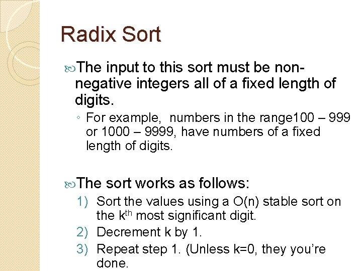
Radix Sort The input to this sort must be nonnegative integers all of a fixed length of digits. ◦ For example, numbers in the range 100 – 999 or 1000 – 9999, have numbers of a fixed length of digits. The sort works as follows: 1) Sort the values using a O(n) stable sort on the kth most significant digit. 2) Decrement k by 1. 3) Repeat step 1. (Unless k=0, they you’re done.

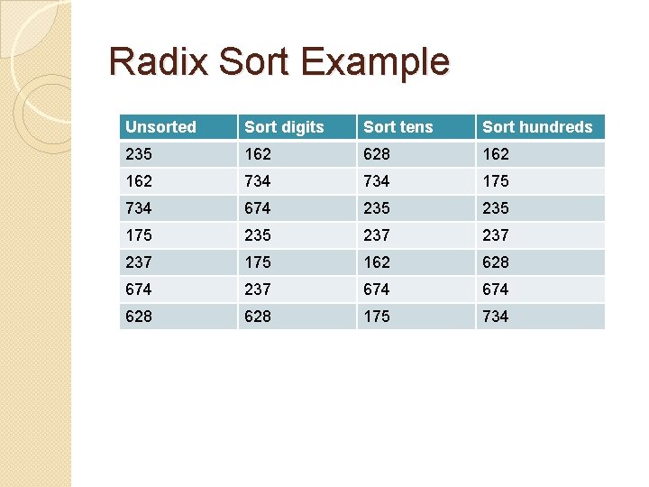
Radix Sort Example Unsorted Sort digits Sort tens Sort hundreds 235 162 628 162 734 175 734 674 235 175 237 237 175 162 628 674 237 674 628 175 734

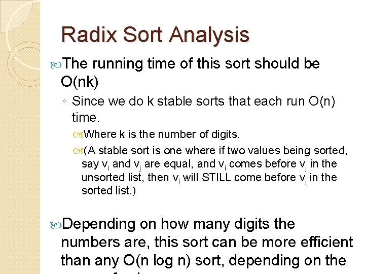
Radix Sort Analysis The running time of this sort should be O(nk) ◦ Since we do k stable sorts that each run O(n) time. Where k is the number of digits. (A stable sort is one where if two values being sorted, say vi and vj are equal, and vi comes before vj in the unsorted list, then vi will STILL come before vj in the sorted list. ) Depending on how many digits the numbers are, this sort can be more efficient than any O(n log n) sort, depending on the

Radix Sort Question: ◦ Would it work the other way around, namely from most significant digit to least significant digit?

A lower time bound for comparison based sorting Shown on the board