Significance Testing Using Monte Carlo Techniques Willem Landman

Significance Testing Using Monte Carlo Techniques Willem Landman and Tony Barnston

Required Reading n Wilks, D. S. 1995: Statistical Methods in the Atmospheric Sciences. Academic Press, New York, p. 145 -157.

Significance Testing n = testing of hypotheses (see any book on statistical methods) n Two contexts in which hypothesis tests are performed q q parametric (theoretical distribution representation of data) non-parametric (distribution-free, e. g. , resampling procedures)

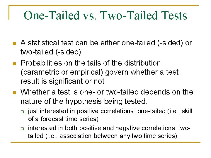
One-Tailed vs. Two-Tailed Tests n n n A statistical test can be either one-tailed (-sided) or two-tailed (-sided) Probabilities on the tails of the distribution (parametric or empirical) govern whether a test result is significant or not Whether a test is one- or two-tailed depends on the nature of the hypothesis being tested: q q just interested in positive correlations: one-tailed (i. e. , skill of a forecast time series) interested in both positive and negative correlations: twotailed (i. e. , association between any two time series)

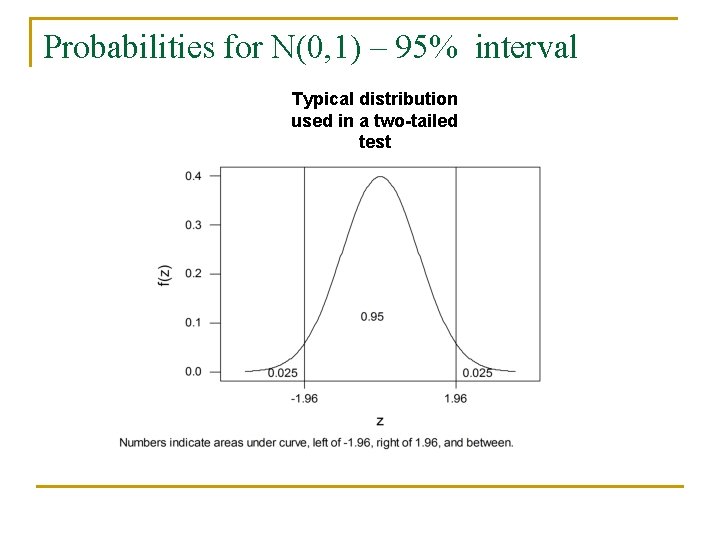
Probabilities for N(0, 1) – 95% interval Typical distribution used in a two-tailed test

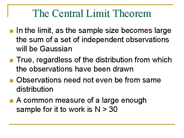
The Central Limit Theorem n n In the limit, as the sample size becomes large the sum of a set of independent observations will be Gaussian True, regardless of the distribution from which the observations have been drawn Observations need not even be from same distribution A common measure of a large enough sample for it to work is N > 30

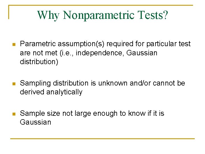
Why Nonparametric Tests? n Parametric assumption(s) required for particular test are not met (i. e. , independence, Gaussian distribution) n Sampling distribution is unknown and/or cannot be derived analytically n Sample size not large enough to know if it is Gaussian

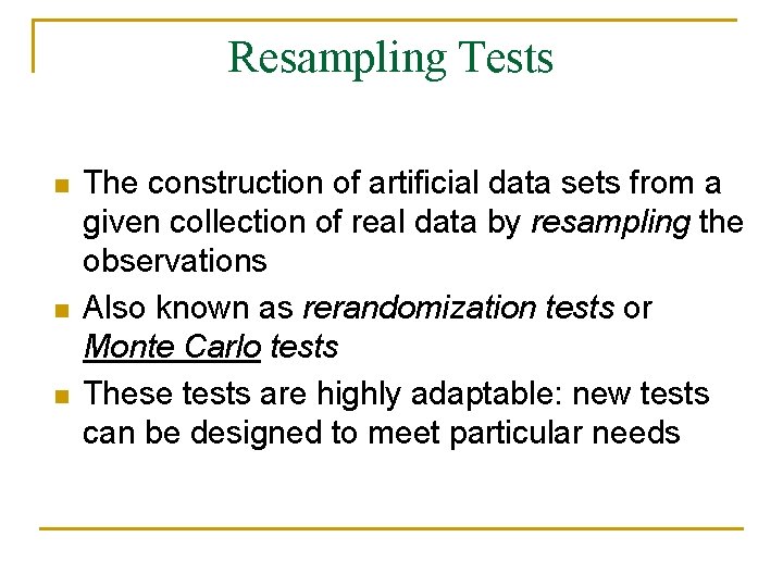
Resampling Tests n n n The construction of artificial data sets from a given collection of real data by resampling the observations Also known as rerandomization tests or Monte Carlo tests These tests are highly adaptable: new tests can be designed to meet particular needs

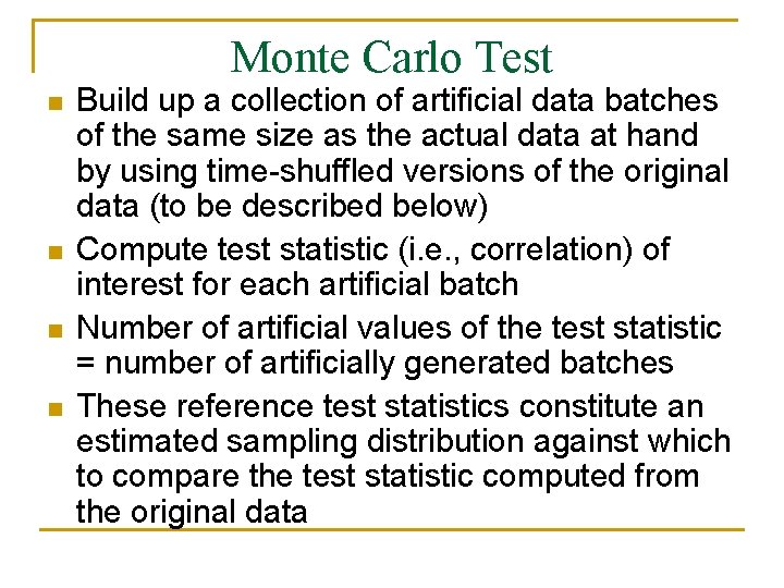
Monte Carlo Test n n Build up a collection of artificial data batches of the same size as the actual data at hand by using time-shuffled versions of the original data (to be described below) Compute test statistic (i. e. , correlation) of interest for each artificial batch Number of artificial values of the test statistic = number of artificially generated batches These reference test statistics constitute an estimated sampling distribution against which to compare the test statistic computed from the original data

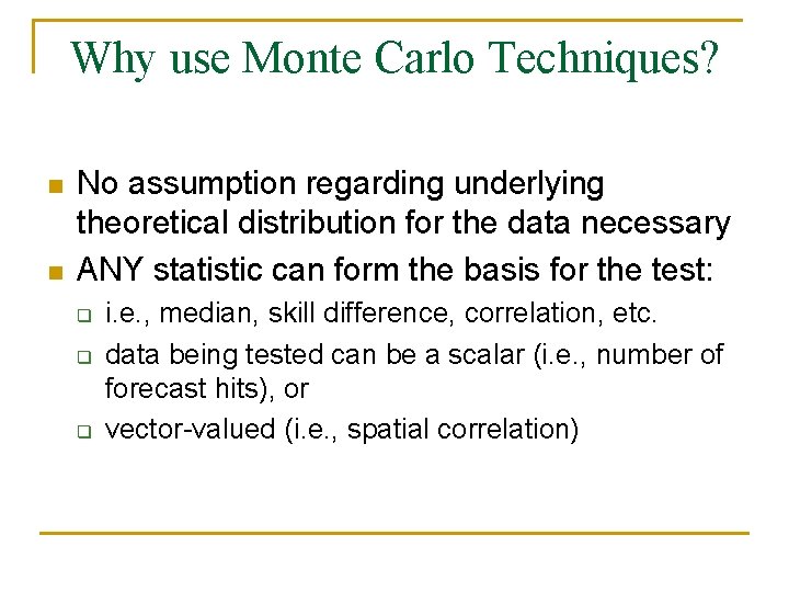
Why use Monte Carlo Techniques? n n No assumption regarding underlying theoretical distribution for the data necessary ANY statistic can form the basis for the test: q q q i. e. , median, skill difference, correlation, etc. data being tested can be a scalar (i. e. , number of forecast hits), or vector-valued (i. e. , spatial correlation)

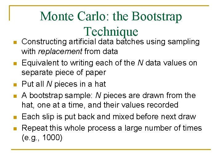
Monte Carlo: the Bootstrap Technique n n n Constructing artificial data batches using sampling with replacement from data Equivalent to writing each of the N data values on separate piece of paper Put all N pieces in a hat A bootstrap sample: N pieces are drawn from the hat, one at a time, and their values recorded Each slip is put back and mixed before next draw Repeat this whole process a large number of times (e. g. , 1000)

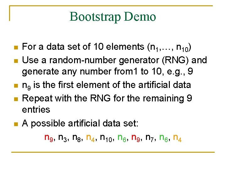
Bootstrap Demo n n n For a data set of 10 elements (n 1, …, n 10) Use a random-number generator (RNG) and generate any number from 1 to 10, e. g. , 9 n 9 is the first element of the artificial data Repeat with the RNG for the remaining 9 entries A possible artificial data set: n 9, n 3, n 8, n 4, n 10, n 6, n 9, n 7, n 6, n 4

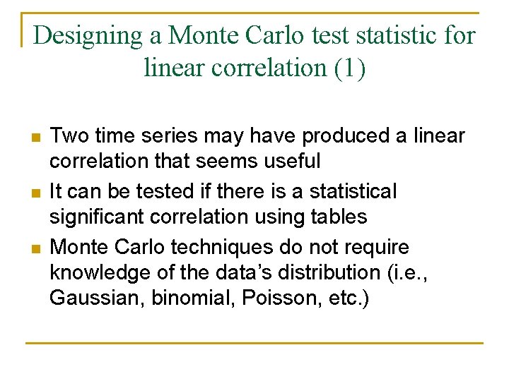
Designing a Monte Carlo test statistic for linear correlation (1) n n n Two time series may have produced a linear correlation that seems useful It can be tested if there is a statistical significant correlation using tables Monte Carlo techniques do not require knowledge of the data’s distribution (i. e. , Gaussian, binomial, Poisson, etc. )

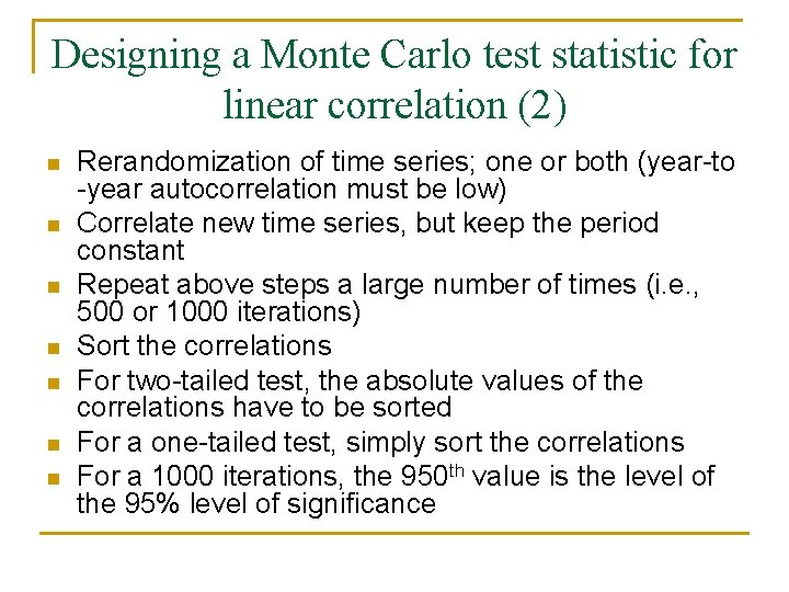
Designing a Monte Carlo test statistic for linear correlation (2) n n n n Rerandomization of time series; one or both (year-to -year autocorrelation must be low) Correlate new time series, but keep the period constant Repeat above steps a large number of times (i. e. , 500 or 1000 iterations) Sort the correlations For two-tailed test, the absolute values of the correlations have to be sorted For a one-tailed test, simply sort the correlations For a 1000 iterations, the 950 th value is the level of the 95% level of significance

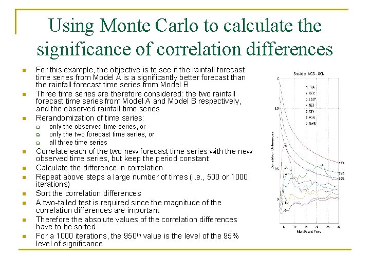
Using Monte Carlo to calculate the significance of correlation differences n n n For this example, the objective is to see if the rainfall forecast time series from Model A is a significantly better forecast than the rainfall forecast time series from Model B Three time series are therefore considered: the two rainfall forecast time series from Model A and Model B respectively, and the observed rainfall time series Rerandomization of time series: q q q n n n n only the observed time series, or only the two forecast time series, or all three time series Correlate each of the two new forecast time series with the new observed time series, but keep the period constant Calculate the difference in correlation Repeat above steps a large number of times (i. e. , 500 or 1000 iterations) Sort the correlation differences A two-tailed test is required since the magnitude of the correlation differences are important Therefore the absolute values of the correlation differences have to be sorted For a 1000 iterations, the 950 th value is the level of the 95% level of significance

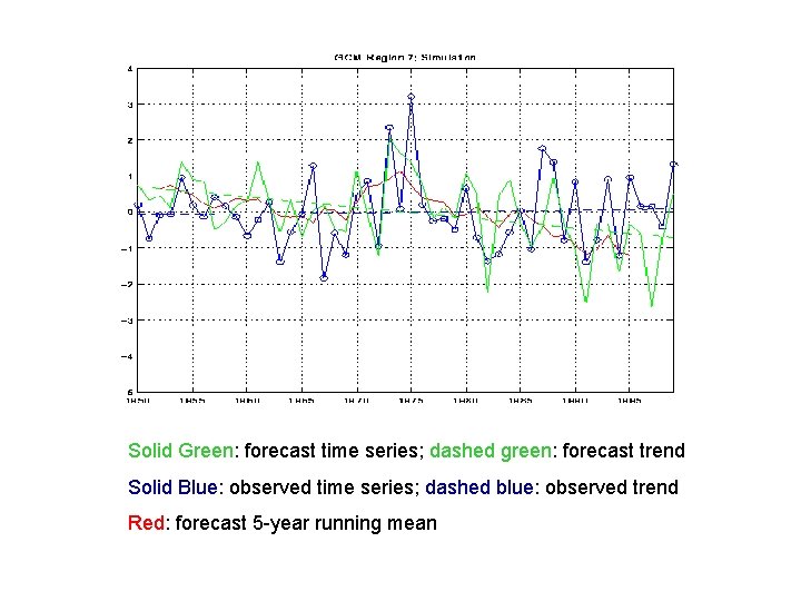
Solid Green: forecast time series; dashed green: forecast trend Solid Blue: observed time series; dashed blue: observed trend Red: forecast 5 -year running mean

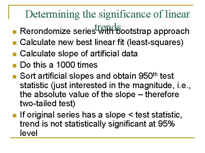
n n n Determining the significance of linear Rerondomize seriestrends with bootstrap approach Calculate new best linear fit (least-squares) Calculate slope of artificial data Do this a 1000 times Sort artificial slopes and obtain 950 th test statistic (just interested in the magnitude, i. e. , the absolute value of the slope – therefore two-tailed test) If original series has a slope < test statistic, trend is not statistically significant at 95% level

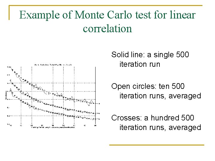
Example of Monte Carlo test for linear correlation Solid line: a single 500 iteration run Open circles: ten 500 iteration runs, averaged Crosses: a hundred 500 iteration runs, averaged

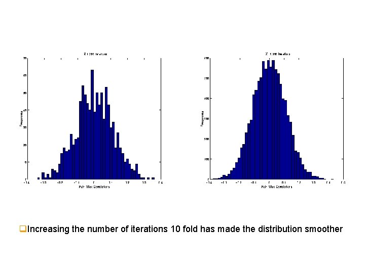
q. Increasing the number of iterations 10 fold has made the distribution smoother

Field Significance and Multiplicity n n n Special problems with statistical tests involving atmospheric fields – testing for pattern significance Positive grid-point-to-grid-point correlation of underlying data produces statistical dependence among local tests Multiplicity: the problem when the results of multiple independent significant tests are jointly evaluated

Stating the problem of Multiplicity through an example n n Say we want to see if there is a significant pattern in the association (correlation) between the Nino 3. 4 index and an area (100 grid points) over the southern Indian Ocean Local tests at each southern Indian Ocean grid-point indicate 8 of the 100 are significant at the 95% level It may be supposed that, since 5% of 100 is 5, getting 8 locally significant correlations is evidence of field significance The following example suggests that this assumption is flawed

…and… …after only a few rerandomization of the rainfall time series…

Using a Monte Carlo approach, it was possible to design a rerandomized rainfall time series that produced an El Niño type spatial pattern in the oceans. Clearly the real association between SON SSTs and the series of random numbers is zero (!!!), but the substantial grid-point-to-grid-point correlation among the SON SSTs yields spatial coherent areas of chance sample correlation that are deceptively high (due to the high spatial correlations the spatial degrees of freedom is far less than the number of grid-points).

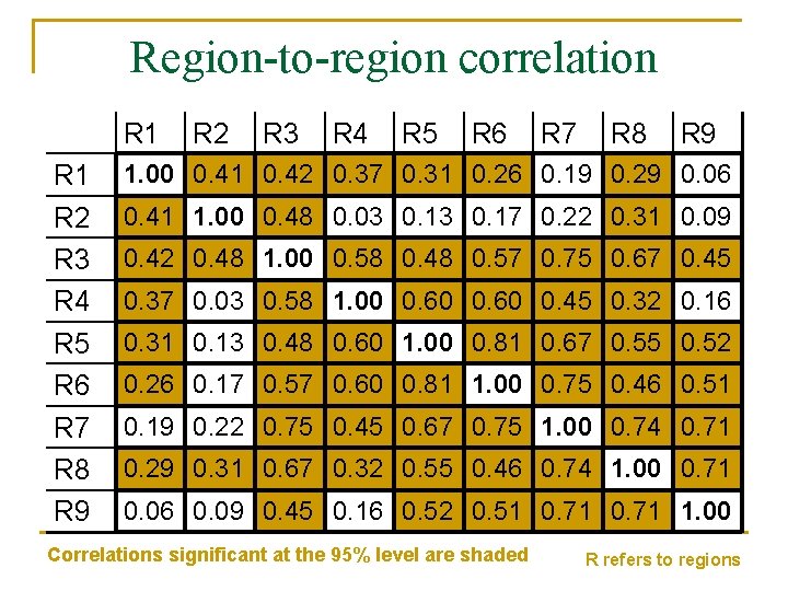
Another example of multiplicity and its solution n n An index of the eastern equatorial Pacific Ocean correlates well with concurrent seasonal rainfall indices of 9 contiguous regions over 50 seasons Local significance tests show significant correlations (95% level) between index and regional rainfall for 7 of the 9 regions However, there are positive region-to-region correlations found in the seasonal rainfall of the regions (see next slide) The question: is getting 7 local significant values significant?

Region-to-region correlation R 1 R 2 R 3 R 4 R 5 R 6 R 7 R 8 R 9 1. 00 0. 41 0. 42 0. 37 0. 31 0. 26 0. 19 0. 29 0. 06 0. 41 1. 00 0. 48 0. 03 0. 17 0. 22 0. 31 0. 09 0. 42 0. 48 1. 00 0. 58 0. 48 0. 57 0. 75 0. 67 0. 45 0. 37 0. 03 0. 58 1. 00 0. 60 0. 45 0. 32 0. 16 0. 31 0. 13 0. 48 0. 60 1. 00 0. 81 0. 67 0. 55 0. 52 0. 26 0. 17 0. 57 0. 60 0. 81 1. 00 0. 75 0. 46 0. 51 0. 19 0. 22 0. 75 0. 45 0. 67 0. 75 1. 00 0. 74 0. 71 0. 29 0. 31 0. 67 0. 32 0. 55 0. 46 0. 74 1. 00 0. 71 0. 06 0. 09 0. 45 0. 16 0. 52 0. 51 0. 71 1. 00 Correlations significant at the 95% level are shaded R refers to regions

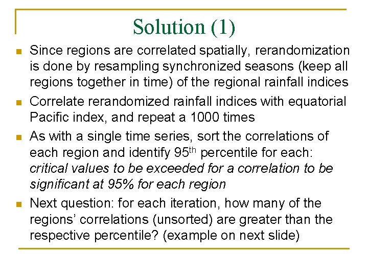
Solution (1) n n Since regions are correlated spatially, rerandomization is done by resampling synchronized seasons (keep all regions together in time) of the regional rainfall indices Correlate rerandomized rainfall indices with equatorial Pacific index, and repeat a 1000 times As with a single time series, sort the correlations of each region and identify 95 th percentile for each: critical values to be exceeded for a correlation to be significant at 95% for each region Next question: for each iteration, how many of the regions’ correlations (unsorted) are greater than the respective percentile? (example on next slide)

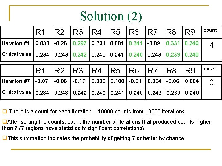
Solution (2) R 1 R 2 R 3 R 4 R 5 R 6 R 7 0. 297 0. 201 0. 001 0. 341 -0. 09 R 8 R 9 Iteration #1 0. 030 -0. 26 Critical value 0. 234 0. 243 0. 242 0. 240 0. 241 0. 240 0. 243 0. 239 0. 240 R 5 R 6 R 7 0. 331 0. 240 R 1 R 2 R 3 R 4 R 8 Iteration #7 -0. 06 -0. 17 0. 096 0. 180 -0. 01 Critical value 0. 234 0. 243 0. 242 0. 240 0. 241 0. 240 0. 243 0. 239 0. 240 0. 004 -0. 06 R 9 0. 064 count 0 q There is a count for each iteration – 10000 counts from 10000 iterations q. After sorting the counts, count the number of iterations that produced counts higher than 7 (7 regions have statistically significant correlations) q. This summation indicates the probability of getting 7 or better by chance

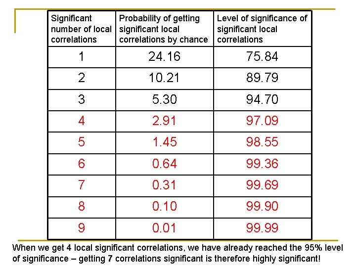
Significant Probability of getting Level of significance of number of local significant local correlations by chance correlations 1 24. 16 75. 84 2 10. 21 89. 79 3 5. 30 94. 70 4 2. 91 97. 09 5 1. 45 98. 55 6 0. 64 99. 36 7 0. 31 99. 69 8 0. 10 99. 90 9 0. 01 99. 99 When we get 4 local significant correlations, we have already reached the 95% level of significance – getting 7 correlations significant is therefore highly significant!