Session 3 Experiments on Individual Preference Chris Starmer

Session 3: Experiments on Individual Preference Chris Starmer TSU Short Course in Experimental and Behavioural Economics, 5 -9 November 2012

Location of Slideshows http: //www. tsu. edu. ge/ge/facultie s/economics/main/

Background • At heart of modern economics are assumptions about preferences – Economics: the ‘theory of Choice’ and preferences explain choice • Economic theories assume people behave as is they have “well-behaved preferences”

Well-behaved? • Individuals can rank any pair of alternatives • Rankings are: – stable - transitive (if A prf B; B prf C then A prf C) - Context free - Depend only on objective features of decision - Don’t depend on how they are measured

Today - Two ‘Anomalies’ • The Endowment Effect • The Preference Reversal Phenomenon • At face value – both provide some challenge to these conventional preference assumptions

Part I THE ENDOWMENT EFFECT

Part 1 – the Endowment Effect • First observed as anomaly in widely used public policy tool – (‘CVM’ on next slide) – later in parallel experimental evidence • I will introduce the anomaly • Discuss three competing interpretations • & Illustrates some experiments used to tease them apart

What is CVM? • CVM = Contingent Valuation Methodology • Survey methodology • Valuing non-marketed goods – public goods • e. g. environment, value of changes in risk • Widely used in public decision making

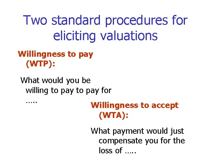
Two standard procedures for eliciting valuations Willingness to pay (WTP): What would you be willing to pay for …. . Willingness to accept (WTA): What payment would just compensate you for the loss of …. .

For general discussion of CVM methods see…. • Hanley, N. (1989) "Valuing Non-market Goods Using Contingent Valuation" Journal of Economic Surveys , 1989, vol. 3, issue 3, pages 235 -52.

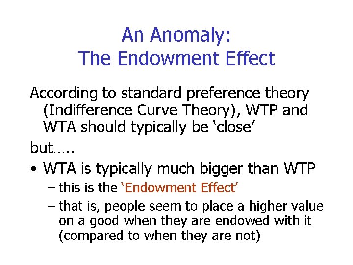
An Anomaly: The Endowment Effect According to standard preference theory (Indifference Curve Theory), WTP and WTA should typically be ‘close’ but…. . • WTA is typically much bigger than WTP – this is the ‘Endowment Effect’ – that is, people seem to place a higher value on a good when they are endowed with it (compared to when they are not)

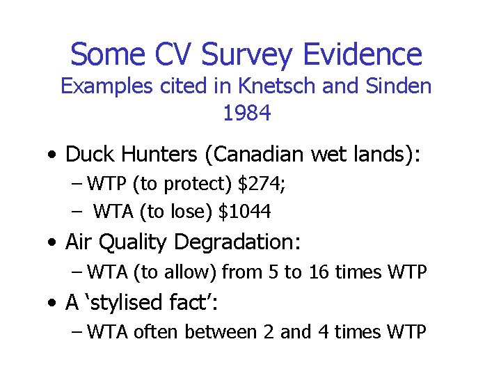
Some CV Survey Evidence Examples cited in Knetsch and Sinden 1984 • Duck Hunters (Canadian wet lands): – WTP (to protect) $274; – WTA (to lose) $1044 • Air Quality Degradation: – WTA (to allow) from 5 to 16 times WTP • A ‘stylised fact’: – WTA often between 2 and 4 times WTP

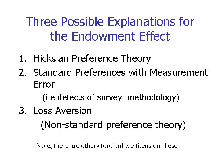
Three Possible Explanations for the Endowment Effect 1. Hicksian Preference Theory 2. Standard Preferences with Measurement Error (i. e defects of survey methodology) 3. Loss Aversion (Non-standard preference theory) Note, there are others too, but we focus on these

Explaining the Endowment Effect Can it be explained by standard preference theory? (i. e. Indifference Curve Analysis)

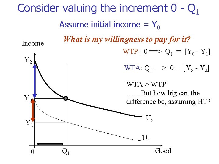
Consider valuing the increment 0 - Q 1 Assume initial income = Y 0 Income What is my willingness to pay for it? WTP: 0 ==> Q 1 = [Y 0 - Y 1] Y 2 WTA: Q 1 ==> 0 = [Y 2 - Y 0] WTA > WTP ……But how big can the difference be, assuming HT? Y 0 U 2 Y 1 U 1 0 Q 1 Good

So WTA > WTP is allowed under standard theory. But how big can the difference be? • Hanemann, AER, 1991 • Theoretically, divergence could be quite large • But, how large is difficult to tell • So, disparity might be explained as consistent with standard preference theory.

Explaining the Endowment Effect The Measurement Error Story

The Measurement Error Story Roughly: • There exist true (WTP/WTA) valuations conforming with standard preference theory • Measured differences between WTP/WTA are too big to be explained by indifference curves • Disparity arises from weaknesses in survey designs which generate Measurement Errors.

Where might the error come from? • Several suggestions: – Hypothetical Bias – Quasi Strategic Reasoning – Misundertsanding of the good • It is common for those taking this line to be especially suspicious of WTA values: – See Arrow, Solow, Portney, Radner, and Schuman (1993) “Report of the NOAA Panel of Contingent Valuation, ” Federal Register, 58: 10 4602 -4614. • Implication for Policy: – improve survey designs – Use WTP over WTA

Explaining the Endowment Effect Loss Aversion Theory

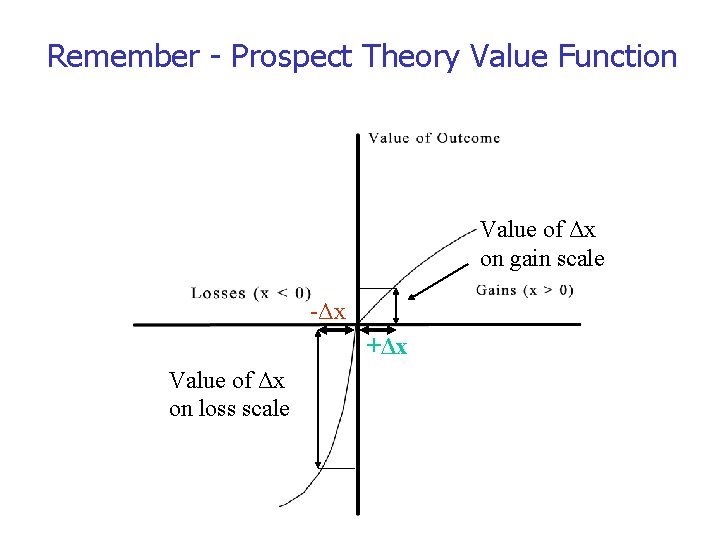
Loss Aversion Theory Roughly: – Human’s respond differently to gains and losses – They are “loss averse” • (ie weigh losses more heavily than gains) – WTA, WTP may be measuring conceptually different things – Which measure is most relevant for public policy evaluation depends on what you are trying to measure

Loss Aversion Theory • Consider example theory with Loss Aversion built in……

Remember - Prospect Theory Value Function Value of Δx on gain scale -Δx +Δx Value of Δx on loss scale

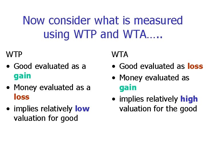
Now consider what is measured using WTP and WTA…. . WTP • Good evaluated as a gain • Money evaluated as a loss • implies relatively low valuation for good WTA • Good evaluated as loss • Money evaluated as gain • implies relatively high valuation for the good

Using Experiments to Evaluate Competing Explanations

Example 1 Knetsch and Sinden, QJE, 1984

K+S • Test Error Theory – Seek to rule out misunderstanding of good – Hypothetical bias • By confronting individuals with: – more realistic/easily understood choice options – choices that have real and immediate consequences for choosers

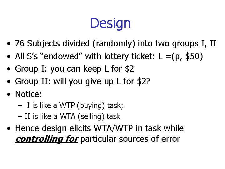
Design • • • 76 Subjects divided (randomly) into two groups I, II All S’s “endowed” with lottery ticket: L =(p, $50) Group I: you can keep L for $2 Group II: will you give up L for $2? Notice: – I is like a WTP (buying) task; – II is like a WTA (selling) task • Hence design elicits WTA/WTP in task while controlling for particular sources of error

Hypothesis • K & S assume wealth effects are negligible. – a potential weakness of their design? • Given this assumption, – standard preference theory implies that the prob. a subject plays the lottery is the same for GI and GII

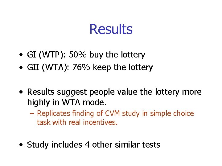
Results • GI (WTP): 50% buy the lottery • GII (WTA): 76% keep the lottery • Results suggest people value the lottery more highly in WTA mode. – Replicates finding of CVM study in simple choice task with real incentives. • Study includes 4 other similar tests

Example 2 Knetsch, AER, 1989

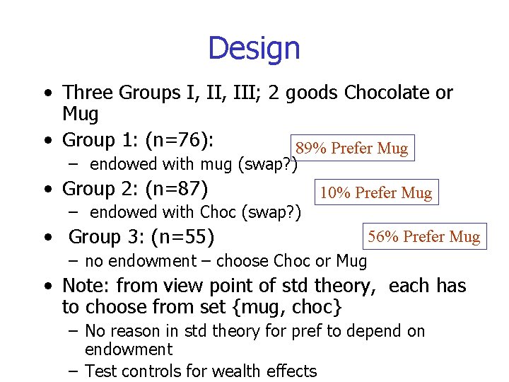
Design • Three Groups I, III; 2 goods Chocolate or Mug • Group 1: (n=76): 89% Prefer Mug – endowed with mug (swap? ) • Group 2: (n=87) – endowed with Choc (swap? ) 10% Prefer Mug • Group 3: (n=55) 56% Prefer Mug – no endowment – choose Choc or Mug • Note: from view point of std theory, each has to choose from set {mug, choc} – No reason in std theory for pref to depend on endowment – Test controls for wealth effects

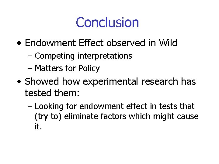
Conclusion • Endowment Effect observed in Wild – Competing interpretations – Matters for Policy • Showed how experimental research has tested them: – Looking for endowment effect in tests that (try to) eliminate factors which might cause it.

Session 3 - Part II

Background • The Preference Reversal Phenomenon (PR) – First observed by Psychologists in 1970 s – Later noticed by Economists • Challenge to basic propositions about preferences • Phases of Investigation – First sightings – Is it a robust/replicable phenomenon • Or an ‘artefact’ of poor experimental design – Developing new explanations – Testing new explanations

Route Map – What is PR – Possible explanations • Faulty experimental design (two waves) • Psychological process theories • Non-transitive preference theory

Preference reversal • A tendency for an individual’s ranking of two alternatives to depend (in a predictable way) on the procedure used to elicit it. – Alternatives might be • Consumptions goods, Government policies • That’s odd (to an economist) because! – Preference theory begins with the assumption that individuals can RANK alternatives – Which do you prefer A or B • Either A pref to B; B pref to A or A ~ B • Alternatively, it is traditional to assume that individuals’ preferences are ‘procedure invariant’ – Don’t change according to how you measure them

Reading Chris Starmer (2008) "Preference Reversal" New Palgrave Dictionary of Economics (2 nd Edition). Copy on TSU web

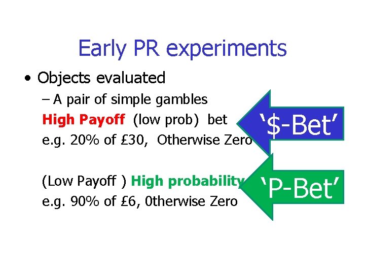
Early PR experiments • Objects evaluated – A pair of simple gambles High Payoff (low prob) bet e. g. 20% of £ 30, Otherwise Zero ‘$-Bet’ (Low Payoff ) High probability e. g. 90% of £ 6, 0 therwise Zero ‘P-Bet’

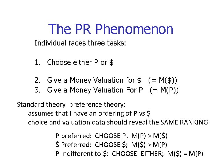
The PR Phenomenon Individual faces three tasks: 1. Choose either P or $ 2. Give a Money Valuation for $ (= M($)) 3. Give a Money Valuation For P (= M(P)) Standard theory preference theory: assumes that I have an ordering of P vs $ choice and valuation data should reveal the SAME RANKING P preferred: CHOOSE P; M(P) > M($) $ Preferred: CHOOSE $; M($) > M(P) P Indifferent to $: CHOOSE EITHER; M($) = M(P)

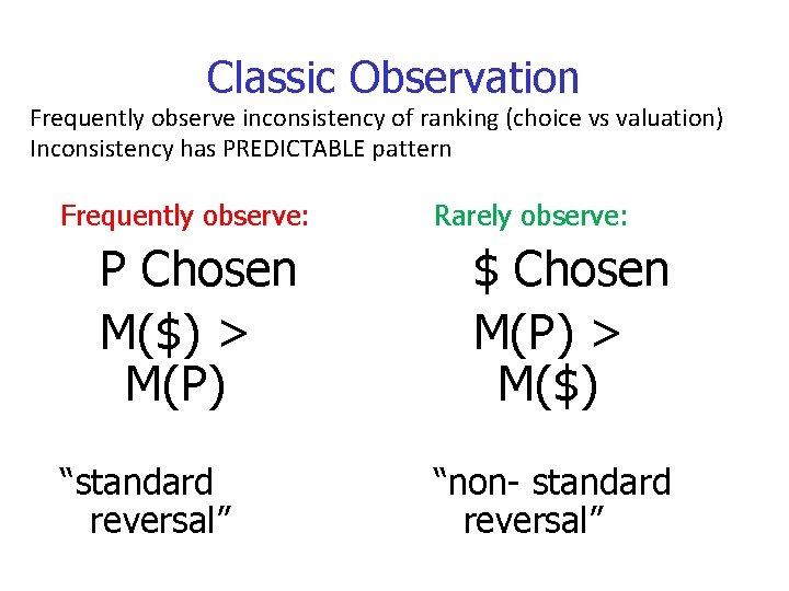
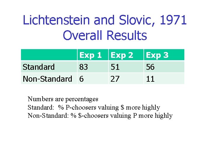
Classic Observation Frequently observe inconsistency of ranking (choice vs valuation) Inconsistency has PREDICTABLE pattern Frequently observe: P Chosen M($) > M(P) “standard reversal” Rarely observe: $ Chosen M(P) > M($) “non- standard reversal”

Lichtenstein and Slovic, 1971 Overall Results Exp 1 Standard 83 Non-Standard 6 Exp 2 51 27 Exp 3 56 11 Numbers are percentages Standard: % P-choosers valuing $ more highly Non-Standard: % $-choosers valuing P more highly

Testing Robustness of PR Grether and Plott, – American Economic Review, 1979 PR potentially important for economics – If PR is robust it would be a major challenge • undermine assumption of optimizing behaviour • Even in a very simple environment But Grether and Plott were sceptical Raised doubts about reliability/interpretation of previous studies

Testing Robustness of PR Propose 13 possible limitation of previous experiments including: Poor Incentives Subject Confusion Experimenters were psychologists!. . Run new experiments: • “. . . all theories for which we exercised control can be rejected as explanations of the phenomenon”

Since then, lots more studies See C. Seidl Review in Journal of Economic Surveys 2002.

Not just a lab phenomenon • Casino Gambling – Lichtenstein and Slovic, Replicate PR with gamblers at Las Vegas Casino

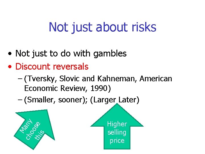
Not just about risks • Not just to do with gambles • Discount reversals Ma ch ny oo th se is – (Tversky, Slovic and Kahneman, American Economic Review, 1990) – (Smaller, sooner); (Larger Later) Higher selling price

Broader Significance of PR • Challenge to basic theoretical assumption • Practical Significance – E. g. Public policy evaluation – Choosing among alternative interventions – Often use estimates of money values • ‘contingent valuation methodology’ – Willingness to pay; willingness to accept

Contingent Valuation Example • Consider plans for new road, 2 poss routes: – both have –ve environmental consequences – Route A: destruction site of special scientific interest – Route B: damage to particularly attractive landscape – Assess willingness to accept (compensation) • That is MONEY VALUATION – Select according to smaller WTA • But would same be selected via choice? • Do WTA money values correctly represent preferences? • PR seeds doubt about that • Need to understand what lies behind PR

Explaining PR • Incentive Mechanisms • Psychological ‘process’ theory • Non-Transitive Preferences

Incentive mechanisms • Large/Specialist literature – PR explained as consequence of: • Non-standard preferences (non-expected utility) • Interacting with features of experimental incentive mechanisms • I wont go into detail but: – PR is reproduced in experiments that rule out this interpretation (See Seidl 2002) • These explanations largely eliminated

Psychological Process Theories • Decisions not (fully) determined by pre-existing preferences • Individualsconstruct decisions – different decision modes (e. g. choice/valuation) may invoke different decision processes. – can lead to different outcomes of choice/valuation – That is preferences do not satisfy PROCEDURE INVARIANCE • Many such theories: – One example • Anchoring and adjustment hypothesis

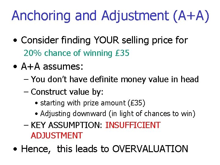
Anchoring and Adjustment (A+A) • Consider finding YOUR selling price for 20% chance of winning £ 35 • A+A assumes: – You don’t have definite money value in head – Construct value by: • starting with prize amount (£ 35) • Adjusting downward (in light of chances to win) – KEY ASSUMPTION: INSUFFICIENT ADJUSTMENT • Hence, this leads to OVERVALUATION

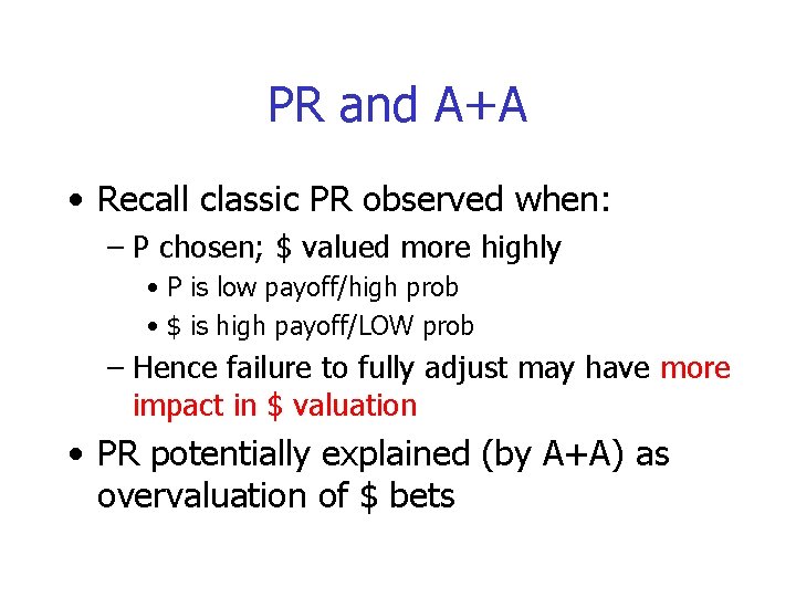
PR and A+A • Recall classic PR observed when: – P chosen; $ valued more highly • P is low payoff/high prob • $ is high payoff/LOW prob – Hence failure to fully adjust may have more impact in $ valuation • PR potentially explained (by A+A) as overvaluation of $ bets

PR as Non-Transitive Preference Regret Theory

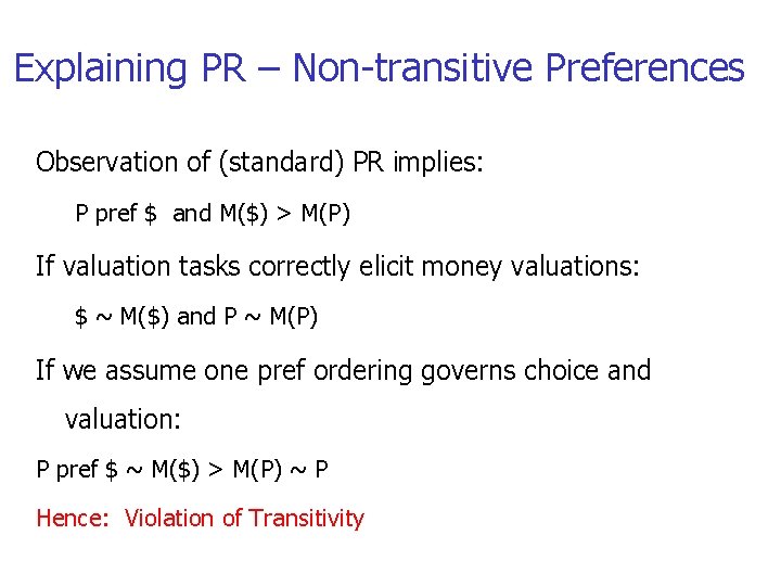
Explaining PR – Non-transitive Preferences Observation of (standard) PR implies: P pref $ and M($) > M(P) If valuation tasks correctly elicit money valuations: $ ~ M($) and P ~ M(P) If we assume one pref ordering governs choice and valuation: P pref $ ~ M($) > M(P) ~ P Hence: Violation of Transitivity

Large Literature • Testing explanations of PR • Some support for – Psych process theories – Intransitivity – And more • Probably multiple mechanisms at work in generation of PR

Conclusions • Both EE and PR create doubt about basic preference assumptions • Both appear robust phenomena • Both have applied/policy significance • Some progress made in explaining them • Suggest – Multiple causal factors – More psychological interpretation of choice

Questions? 60